LibreOffice Calc: Pivot Table Made Easy

This tutorial will show you how to create Pivot Table using LibreOffice Calc -- the complete, free spreadsheet program for everyone. We will learn with examples and pictures by using a simple sales table to create sales report with multiple pivot tables we want. Now let's exercise!

Subscribe to UbuntuBuzz Telegram Channel to get article updates.

What is pivot table?

Pivot table is basically moving a table into another table in different form with filters.

What we will create?

Our goal this time is to make summaries of a data table in Picture 1. It is an imaginary sales data with date, employee, product category, shop, and sales columns. Basically, we will turn the data from Picture 1 below into Picture 2. Finally, you might notice that the employee names involved here are the same as the previous at our Calc Tutorials. As an acknowledgement, this table is adapted from Ellak Course's Example File mentioned at references section (that one with Brigitte, Elen, Fritz and friends).

 Picture 1. Data source

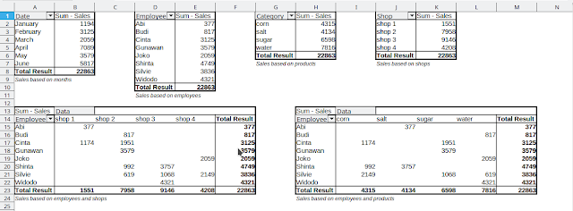
 Picture 2. Pivot tables

How To Use the Filters

A pivot table is typically equipped with one filter or more depicted as a drop down button at each column head. See the difference below.

 Picture 4. Pivot tables with filters selected (notice the color and signs)

To show pivot table like the above, you change the filters by selecting items you want to be displayed. Picture 5 shows the employee filter selections of the three sample tables shown above.

Tips: aside from filtering, filters are also equipped with sorting capabilities. For example, for the date-based pivot table, you can enable filter > Custom sort > select January, February, March ... > data sorted according to month order. You can also select order ascending or descending if you want. See picture 5. 

Step 1. Prepare Data Source

In order to make Pivot Table, you need a data source first. Write Table 1 with Calc and then save it as pivot-table-exercise.ods. This table is called data source.

 Table 1. Data Source

Step 2. Create a basic Pivot Table

1. Select a cell in the source table.  Do not select multiple cell as Calc is able to read your table thoroughly.

2. Go to Insert > Pivot Table > Pivot Table Layout dialog will open.

3. Drag and drop "employee" from right to left under Row fields. See picture 6.

4. Drag and drop "sales" from right to left under Data Fields. See picture 6.

5. Click OK. 

6. Pivot Table created in a new sheet called Pivot Something.

 Picture 6. Pivot Table dialog

Step 3. Pivot Table Created

Pivot table with one criteria will be created in a new sheet.

Explanation: this is the very basic of pivot table, it sums up between employees and their sales respectively and display them without duplicated data. For example, we can say that Cinta's sales is 3125, Shinta's 4749 while Silvie's 3836. This way, computer helps us to calculate them precisely and accordingly without us doing redundant job repeatedly. Using the same method, you can create four pivot tables based on our example:

Employee Sales Table

This table sums up employees and their respective sales. This helps us to examine that Abi is the lowest while Shinta and Widodo are the highest, in sales.

Table 3. Employee sales

Products Category Sales Table

This table sums up products (category) and their respective sales.  This helps us to see quickly that water is the highest while corn and salt are the lowest in sales.

Shop Sales Table

This table sums up shop branches and their respective sales. This helps us to quickly see that shop 1 is the lowest selling, shop 3 is the highest selling.

Table 5. Shop sales

Date Sales Table

This table sums up month (date) and their respective sales. This helps us to see quickly that January is the lowest month while April is the highest month in sales.

Table 6. Date sales

Pivot Table with Two Criteria or More

1. Repeat step 1 to 3 above with one more criteria into Row Fields.

2. Alternatively, you may instead put one criteria into Row Fields, and put another one into Column Fields.

3. A new pivot table created.

Table 7. Pivot table with two criteria

Table 8. Same pivot table but with Products Category as Column Fields

Explanation: pivot table above displays a summary of sales according to employees and category. From that, for example, we can say that Abi sells only salt, Budi sells only water, Cinta sells corn and sugar, while Silvie sells corn, sugar and water. We can also say, that Cinta's corn's 1174, Shinta's corn's 992 while Silvie's corn's 2149. Using the same method, you can create many combination of pivot tables as shown below:

Employee / Month Sales Table

This table sums up a comparison between employees and months (date) of sales.  This helps us to see in two ways, at the same time, total results of employee and month. For example, employee Silvie's total is 3836 while month April's total is 7089.

  Table 9. Sales by employee / month

Employee / Shop Sales Table

This table sums up a map between employees and shops in sales. This helps us observe two things at the same time, for example, total results of employee and shop. Further, let's say that employee Cinta's total is 3125 while branch Shop 2's total is 7958.

Table 10. Sales by employee / shop

Employee / Products Table

This table sums up a map of employees and their products (category) sales. This helps us to observe in two ways at the same time between employee and product total results. For example, we can say that employee Silvie's total is 3836 while product category Sugar's total is 6598.

Employee / Criteria Table, Inverted Position

You can also switch between row and column position of any field item. For example, this is the same table as Employee / Month above, but by putting Employee to Column Field and Date to Row Field in the Pivot Table dialog. As a result, here employees became columns and month became rows, especially now they can be filtered more easily. Compare the difference.

Source: Ubuntu Buzz !