This powerful programming language for scientific computing has an extensive library of functions for generating waves of various shapes.

The following section explains using the square() function to generate square waves. In the following, we will show you practical examples and pictures of how to create square waves with different parameters and display them graphically in the MATLAB environment.

MATLAB Square Function Syntax

MATLAB Square Function Description

MATLAB square() function generates square waves from time vectors or matrices. This function also allows you to set duty cycle values, often used in electronic models to control DC pulse width modulation (PWM) motors. The MATLAB function square() generates a square wave at “x” from the time matrix “t”. The period of the wave generated at “x” is 2pi over the elements of “t”. The output values of “x” are -1 for negative half cycles and 1 for positive half cycles. The duty cycle is set via the “duty” input sending the percentage of the positive cycle entered when the function is called.

What Is It and How To Create a Time Vector To Generate Waves in MATLAB

Before we see how a square wave is generated with this function, we will briefly show you what vectors and time matrices are. They are part of the input arguments of all functions used to create waves, regardless of their form or the function that generates them. The following is a time vector “t” representing one second in duration:

 
It is essential to clarify that a time vector with ten elements corresponds to a sampling rate of 10 Hz and is not recommended in practice. Hence, we make it only as an example so you can see better what we are talking about because of a vector with a sampling of 1Kz. It would consist of 1000 elements displayed on the screen. A low sampling rate would distort the waveform, as shown below:

Next, let’s look at the expression for one of the ways MATLAB creates this kind of regular-interval time vector:

 
So, to generate this vector, we would need to write the following line of code:

How To Create a Square Wave With the MATLAB Square Function

We will create a square wave using the square() function in this example. This wave has a duration of one second, a frequency of 5Hz, and an amplitude of +1, -1. To do this, we first create a time vector “t” of one-second duration with a sampling frequency of 1KHz or intervals of 1ms.

 
Then, we specify the frequency of the wave. The input argument of square() that sets this value is expressed in radians, so we have to convert from Hz to radians or express it in the latter. For practical reasons, it is always better to express frequency in Hz. Therefore, in this example, we will do the conversion as follows:

 
With the time vector “t” created and the frequency “rad” converted to radians, we now call the square() function as follows:

 
To graph the wave in the MATLAB environment, we will use the following functions:

 
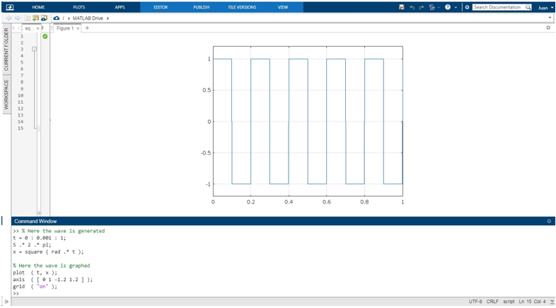
In this case, as the duty cycle input is not used, this value defaults to 50%,. So, square() produces a symmetric wave. Copy and paste the following fragment into the command console to visualize the generated wave.

 
The following image shows the waveform generated by the square() function plotted in the MATLAB environment:

How To Control The Frequency, Amplitude, Duty Cycle, and Sampling Rate When Generating a Wave With the MATLAB square() Function.

This example shows how to control the frequency, amplitude, duty cycle, and sampling rate parameters. For this purpose, we will create a simple console application that will be used to input these values and then automatically graph the wave generated from the input parameters. We will use the prompt() and input() functions to input these parameters through the console. We will store these parameters in the following variables:

s_rate: sampling frequency in Hz

freq: frequency of the wave in Hz

Amp: Amplitude of the wave

d_cycle: duty cycle

These variables are processed respectively to set the parameters “t_sample” in the time vector, the input arguments “rad” and “dc” to the square() function, and the multiplication factor “amp” to adjust the amplitude of the wave.

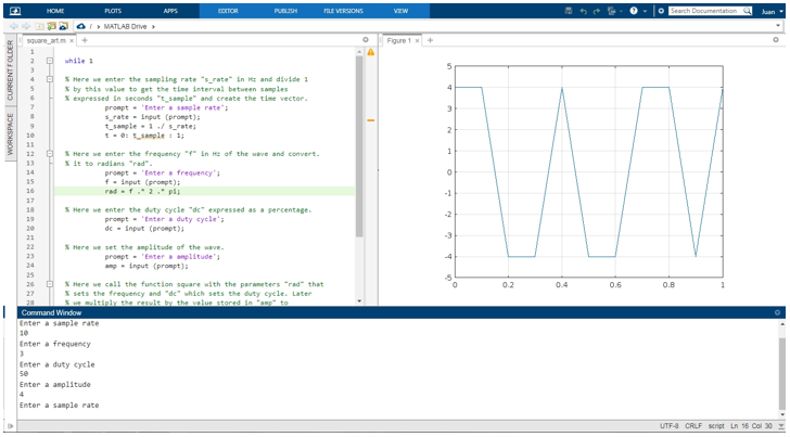
Below, we see the full script for this application. To make it readable, we have divided the code into six blocks, explaining what each of them does in the comments at the beginning.

 
Create a script, paste this code, and press “Run”. To close the application, press Ctrl+c. In the following images, you can see the resulting waves with different parameters entered into the application via the command console:

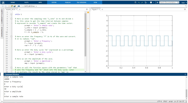
This image corresponds to an 8 Hz wave with a sampling rate of 1Kz, a duty cycle of 50%, and a peak-to-peak amplitude of 2.

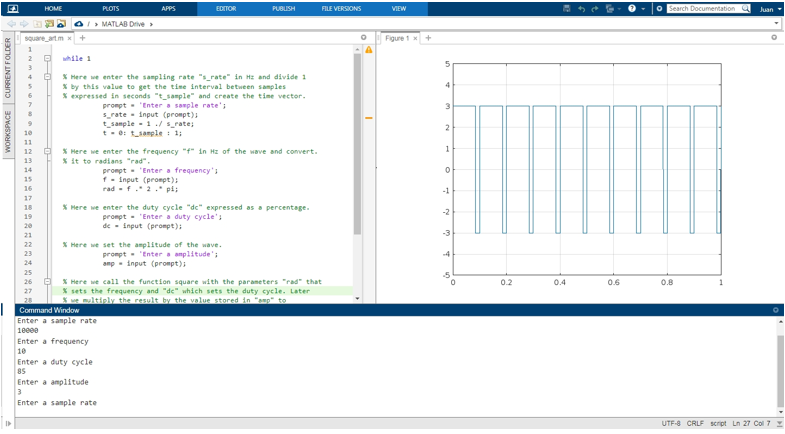
This image corresponds to a 10 Hz wave with a sampling rate of 10Kz, a duty cycle of 85%, and a peak-to-peak amplitude of 6

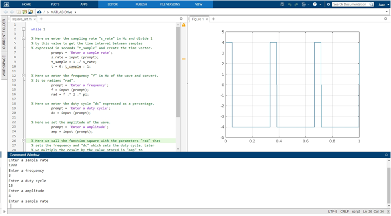
This image corresponds to a 3 Hz wave with a sampling rate of 1Kz, a duty cycle of 15%, and a peak-to-peak amplitude of 8.

Conclusion

This article explained how to generate square waves using the MATLAB function square().
It also includes a brief description of the time vectors and matrices that form the input arguments of this type of function, so you can get a complete understanding of how most of the waveform generators in the Signal Analysis Toolbox in MATLAB work. This article also includes practical examples, graphs, and scripts that show how the square() function works in MATLAB. We hope you found this MATLAB article helpful. See other Linux Hint articles for more tips and information.