SciPy Simpson
In Python, there are many powerful numerical integration methods including the “scipy.integrate.simps()” method which is referred to as “Simpson’s rule integration”. This blog guide will explore the “scipy.integrate.simps()” method and how to use this method in Python using a variety of examples.
What is SciPy Simpson?
The “scipy.integrate.simps()” method is a numerical integration technique based on “Simpson’s rule”. It is used to estimate the definite integral of a function or a dataset by approximating the area under the curve. “Simpson’s rule” is particularly effective for smooth functions and provides accurate results compared to other numerical integration methods.
Syntax
Parameters
In the above syntax:
- The “y” parameter is the value of the function or dataset to be integrated.
- The “x” optional parameter refers to the coordinates corresponding to the values in “y”. If not provided, the integral is assumed to be over a uniform grid.
- Similarly, “dx” is also an optional parameter that indicates the spacing between consecutive elements in “x” and has a default value of “1”.
- The “axis” optional parameter specifies the axis along which the integration is performed. Its default value is assigned to “-1” which indicates/specifies the last axis.
- Lastly, the “even” optional parameter determines how to handle the number of points.
Return Value
The “scipy.integrate.simps()” method returns the estimated value of the definite integral.
Example 1: Calculating the Integral Using the “scipy.integrate.simps()” Method
Let’s start with a simple example to demonstrate the use of the “scipy.integrate.simps()” method in Python:
from scipy import integrate
def f(x):
return x ** 4
x = numpy.linspace(0, 1, 50)
integral = integrate.simps(f(x), x)
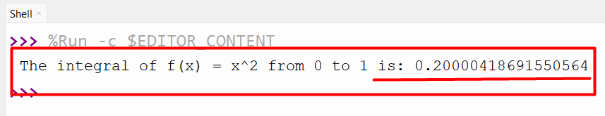
print("The integral of f(x) = x^2 from 0 to 1 is:", integral)
In the above example:
- The “numpy” library and the “integrate” module (from the “scipy” library) are imported/included.
- A simple function named “f(x)” is defined with a return value of “x ** 4”.
- The “numpy.linspace()” function is used to generate “50” equally spaced values between “0” and “1”.
- The “scipy.integrate.simps()” method calculates the integral by taking the return value of the function and the corresponding “x” coordinates as its arguments.
Output
Example 2: Integrating a Dataset With Multiple Dimensions
The “scipy.integrate.simps()” method can also handle datasets with multiple dimensions:
from scipy import integrate
data = numpy.array([[4, 6, 8], [1, 3, 11]])
integral = integrate.simps(data, axis=0)
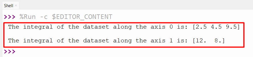
print("The integral of the dataset along the axis 0 is:", integral)
integral_1 = integrate.simps(data, axis=1)
print("\nThe integral of the dataset along the axis 1 is:", integral_1)
In this example:
- Likewise, the “numpy” and “integrate” modules from the “scipy” library are imported.
- The “numpy.array()” method is used to construct a “2-D” array.
- The “integrate.simps()” method takes the “data” i.e., array and the “axis=0” (Vertical Axis) as its arguments, respectively to calculate the integral of each column of the data.
- Similarly the “integrate.simps()” method is utilized again to calculate the integral of each row of the data by taking “data” and “axis=1” as its arguments, respectively.
Output
Conclusion
The “simps()” method of the “SciPy” library is used to compute numerical integration by utilizing “Simpson’s rule”. It is an efficient function that can handle “1” dimensional and multi-dimensional datasets. This Python guide delivered an in-depth guide on “Scipy Simpson” using numerous examples.
Source: linuxhint.com