“ODEs” are equations that relate the rate of change of a particular function with its current value. They are used in many different fields, including engineering, physics, chemistry, and biology. This function is used to solve ordinary differential equations (ODEs). In this Python blog post, we will discuss the “odeint()” function in Python.

What is the “odeint()” Function in Python?

The “odeint()” function of the “scipy.integrate” module can solve a system of ODE/Ordinary Differential Equations by integrating them. This function uses numerical methods to solve ODEs.

Syntax

Parameters

The following parameters are used by the “odeint()” function:

• The “func” parameter is used to calculate the derivative of the given “ODE”.
• The “y0” parameter indicates the initial value of the function.
• The “t” attribute specifies the collection of time points.
• The “args” parameter is a tuple of additional arguments that are passed to the “func” function.
• The “Dfun” parameter specifies a function that calculates the “Jacobian” of the ODE. The “Jacobian” is a matrix that contains the partial derivatives of the ODE with respect to its variables.
• The “full_output” parameter is a boolean value that specifies whether the “odeint()” function should return a tuple containing the solution, the step size, and the error.
• The “jac” parameter refers to a function that calculates the “Jacobian” of the ODE.
• The “options” parameter is a dictionary of options that control the behavior of the “odeint()” function.

Return Value

The “odeint()” function returns a “NumPy” array that contains the solution against the corresponding ODE. The solution is a vector that contains the value of the function at each time point.

Example 1: Solving the Given “ODE” Equation Using the “odeint()” Function

This example solves the below-given “ODE” with the initial condition “y(0) = 3”:

In the above code:

• The “numpy” and “scipy” libraries are imported at the start of the program.
• The user-defined function named “func()” is defined as having two parameters “y” and “t” and retrieves the value of the input ODE.
• The initial value of “y0” is set to “3”.
• The “linspace()” function is utilized to generate an array of “50” numbers evenly spaced from “0” to “5”.
• Next, the “odeint()” function solves the given ODE with the initial condition “y(0) = 3”.
• Lastly, the “odeint()” function returns an array of solutions for each value of “t”.

Output

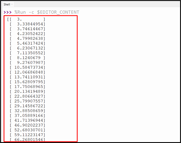
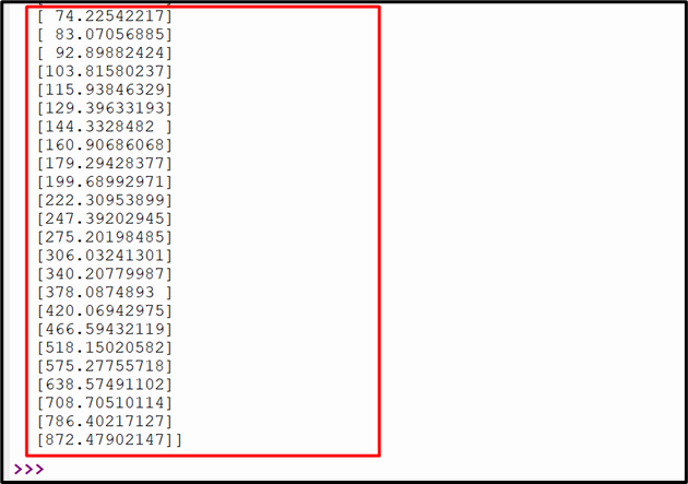
The above output shows the result of the provided “ODE” equation.

Example 2: Plotting the Graph of “odeint()” Function

The below code is used to plot the graph of the discussed function:

According to the above code:

• The code is the same as in the previous example, except for the code for plotting the output in the graph.
• The “plot()” function takes the “t” and “sol” arguments to plot the output of the “odeint()” function in a graph.

Output

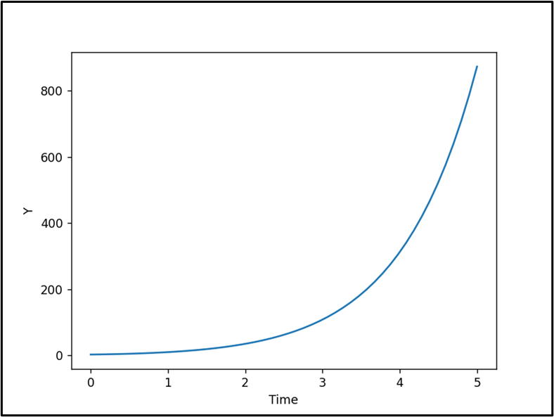
The plot of the “odeint()” function with respect to time has been displayed in the above output.

Conclusion

The purpose of this blog post is to introduce you to the “odeint()” function in Python, which can solve ordinary differential equations (ODEs). “ODEs” describe how a function changes over time based on its current value. This blog demonstrated the working of the SciPy “odient()” function.