SciPy Leastsq
This article will present you with a comprehensive guide on scipy.leastsq() function using numerous examples and via the following contents:
- What is the “scipy.optimize.leastsq” in Python?
- Basic Working of “scipy.optimize.leastsq()” Function
- Fitting a line to data points Using “scipy.optimize.leastsq()” Function
- Using “scipy.optimize.least_squares()” Function
What is the “scipy.optimize.leastsq” in Python?
The scipy.optimize.leastsq() function in Python is utilized to minimize the sum of squares of equations set. This function determines the parameters that minimize/reduce the sum of the squares by solving a nonlinear least squares problem.
Syntax
Parameters
Here:
- The “func” parameter can be used by calling it. It needs an argument in the form of a vector “N” and will give back a floating-point number “M”. It is necessary that “M” is greater than or equal to “N”, and it should not give back NaNs values.
- The “x0” parameter specifies the initial minimization estimate.
- The “args” parameter is a group of values that can be added to the function if needed.
- The optional “Dfun” parameter is utilized to compute the Jacobian of a function with derivatives concerning the rows.
- The optional “FullOutput” parameter retrieves all extra results, and the “ColDerive” optional parameter calculates derivatives down the columns.
- The “f-Tol” optional parameter indicates how much error is allowed in the sum of squares.
Check this official documentation for more info related to the syntax.
Return Value
The scipy.optimize.leastsq() function retrieves a tuple value containing the following output:
- x: This is an array containing the solution (the optimal values of the independent variables)
- info: This is an array containing the estimated covariance matrix of x.
- infodict: This is a dictionary containing optional outputs, such as fvec, fjac, and ipvt.
- message: This is a string containing a message describing why termination occurred.
- ier: This is an integer indicating why termination occurred.
Example 1: Basic Working of “scipy.optimize.leastsq()” Function
Let us understand this by the following example code:
def new_function(x):
return 23*(x-2)**1+4
print( scipy.optimize.leastsq(new_function, 0))
In the above code:
- The “scipy” module with the “optimize.leastsq” function is imported.
- Next, the function called new_function() is defined with one argument. This function returns the value of 23*(x-2)**1+4, which is a linear function with a slope of 23 and an intercept of 50.
- The scipy.optimize.leastsq() function takes the new_function and 0 as arguments. This function uses the least squares method to find the values of x that make new_function(x) as close to zero as possible.
Output
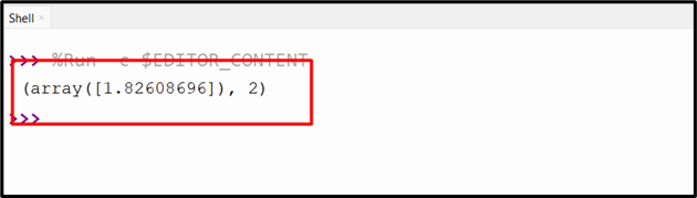
The function returns a tuple of two elements: the first element is an array of the optimal values of x, and the second element is an integer that indicates the status of the optimization process. Here, the best-fit parameters value is “1.826”, and the successful optimization integer value is “2”.
Example 2: Fitting a Line to Data Points Using “scipy.optimize.leastsq()” Function
Here is an example that utilizes the “scipy.optimize.leastsq()” function to fit a line of data points:
import numpy as np
data_x = np.array([0, 1, 2, 3, 4, 5])
data_y = [2.5, 4.7, 6.3, 8.2, 10.1, 11.9]
def linear_function(parameters, x):
return parameters[0] * x + parameters[1]
def calculate_error(parameters, x, y):
return linear_function(parameters, x) - y
initial_parameters = np.array([1.2, 1.8])
res = opt.leastsq(calculate_error, initial_parameters, args=(data_x, data_y))
print(res)
In this example code:
- The “scip.optimize” and “numpy” modules are imported, and the data points to fit are defined as an array.
- Next, the function representing the line and the function representing the error that calculates the difference between the line and the data points is defined.
- Next, we provide an initial guess for the parameters of the line and call leastsq with the error function, the initial guess, and the data points as arguments.
- Finally, we print the optimal parameters for the line.
Output
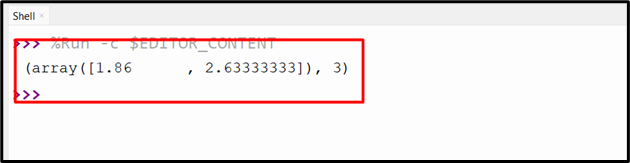
The above output displays two values: the optimal parameters (1.826 & 2.633) and a boolean value (3) that indicates whether the optimization was successful.
Example 3: Using “scipy.optimize.least_squares()” Function
The scipy.optimize.least_squares() function is a Python function that can be used to solve a nonlinear least-squares problem with bounds on the variables. The leastsq() and least_squares() are two functions in the SciPy library that can be used to solve nonlinear least squares problems.
The leastsq() method reduces the sum of squared equations we learned earlier, while least_squares() solve a nonlinear least-squares problem by setting limits on the variables.
Let’s understand the “scipy.optimize.least_squares()” function via the following code:
from scipy import optimize
def custom_function(y):
return np.array([5 * (y[1] - y[0]**2), (0.5 - y[0])])
initial_guess = np.array([2, 2])
result = optimize.least_squares(custom_function, initial_guess)
print('Solution:', result.x)
print('Cost:', result.cost)
print('Optimality:', result.optimality)
Here:
- The first two lines import the scipy.optimize and numpy modules.
- Next, we define a function that takes a NumPy array as input and returns a NumPy array of the same size. The elements of the output array are the squared errors between the data points and function.
- After that, we define the initial guess for the function parameters.
- Lastly, we call the least_squares() function to determine the function’s optimal parameters.
- Here, the least_squares() function takes two parameters: the custom function and the initial guess.
- The least_squares() function returns an object that contains the optimal parameters, the cost of the function, and the optimality of the solution.
Output
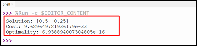
The optimal parameters have been retrieved successfully.
Conclusion
In Python, the “scipy.optimize.leastsq()” function of the “scipy” library is used to find the best-fit line for a set of data points. The “scipy.optimize.leastsq()” function is used to fit the curve data with a given function by applying the least-square minimization technique. We can also utilize the scipy.optimize.least_squares() function to solve a nonlinear least-squares problem by setting limits on the variables. This guide demonstrates details on Python’s “scipy.optimize.leastsq()” function using numerous examples.
Source: linuxhint.com