Many well-known mathematical procedures have built-in functions in Python’s SciPy scientific computing package. The scipy.integrate sub-package includes an integrator for ordinary differential equations as one of the integration techniques. This article will teach you how to utilize the “SciPy Integrate” to solve integration problems using the integration approach. We’ll talk about some related topics as well. These are SciPy integrate, trapezoid SciPy integrate quad, and SciPy integrate simpson. To help you comprehend and use the concepts on your own, we will go through these ideas in detail and with useful programming examples. So, let’s start.

SciPy Integrate Definition

The numerous approaches to Python integration or differential equation issues are all contained in the SciPy submodule scipy.integrate. It has a predetermined purpose and approach for handling integration or differential equation issues. Use the following code to learn about the integration methods supported by this submodule.

 
You will see a detailed output from the previous code. A small section of the produced output is shown below:

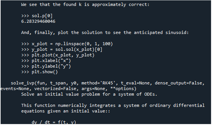
When we scroll through the output, all of this module’s integration and differential methods, techniques, and functions are displayed.

You now have some key information regarding scipy.integrate. Focusing on some programming examples will help. For your benefit, screenshots are also included, and suitable explanations are provided for these examples.

Example 1

We’ll talk about the scipy.integrate.trapz() method in the first example. Using a straightforward Gaussian quadrature of fixed order n, a definite integral is computed using SciPy’s scipy.integrate.trapz technique. You can find the following syntax:

The parameters y, x, dx, and axis are included. The “y” parameter indicates the input array that must be integrated. It must resemble an object from a Python array. The sample points that correspond to the y values make up the “x” parameter. The sample points are required to be evenly spaced apart by dx. It is in the case if x is not specified. When x is None, the optional scaler parameter dx represents the distance between sample locations. The initial setting is 1. The optional number in the axis parameter indicates the axis along which to integrate.

Now, let’s discuss the example here. The code is attached below. As you can see, it is a very simple code and can easily be understood.

First, we imported NumPy and the integrate library. We then passed the array having values [4, 5 ,6] to the scipy.integrate.trapz() method. It integrates the created array by using the trapezoidal rule. Finally, the output is displayed using the print(trap_method) statement.

 
Below is the result of the executed code:

Example 2

This is another example from this post in which we will discuss using scipy.integrate.fixed quad to compute the order 5 Gaussian quadrature approximation. Essentially, the function calculates a definite integral. It is done with Gaussian quadrature of fixed order n. The syntax is shown below:

The method has five parameters: func, a, b, args, and n. The “func” parameter represents the function that will be integrated using the Gaussian quadrature. The function should support vector inputs. The array that we get after integrating a vector-valued function must share the shape (…, len(x)). The “a” parameter indicates the lowest limit of integration. The float type is present. The “b” parameter constrains the maximum integration. The float type is present. A list of additional arguments passed to func in the form of the optional parameter called “args”. The order of the Gaussian quadrature, n, is the last parameter. The standard setting is 5.

Let’s talk about code. In this example, we’ll use SciPy to compute the function f(x) = sin(x )’s 5 Gaussian quadrature approximation. Over the fixed range of 0-pi/4, use the integrate.fixed quad technique.

Let’s figure out the code line-by-line. At the start, we imported the NumPy library. After that, we added the integrated sub package from the SciPy library. Following that, we utilized the numpy.sin() method as the main program that we are going to integrate. In this function, 1 and 4 are passed as parameters, and the limit of the integration is set to 3, which is another parameter indicated as “n=3” in the code. This is done inside the print statement, and its result is shown below:

 
Refer to the generated output that is attached here.

Example 3

The SciPy contains a method called simpson() that estimates an integral’s value. The scipy.integrate submodule includes this method. Here is the following syntax for using it in Python:

The syntax includes five parameters. These are y(array_data), x(array_data), dx(scalar), axis(int), and even(string).

The array that should be integrated as input is by the “y(array data) parameter”. The sample points that correspond to the y values are specified using the “x(array data)” option. When the x is not used, the “dx(scalar)” is used to describe the distance between sample locations. The “Axis(int)” parameter specifies which axis will be used for the integration. The trapezoidal rule on the result of the first and last interval is specified by the “even(string)” parameter.

Now, let’s consider an example program. As seen in the code, we have loaded the necessary module. After that, we created an array of data. Then we created the sample points. Following that, we calculated the integration using the simpson() method. The integral value of the array is displayed in the output, and the provided sample points are 104.5.

 
You can see the following output, and you can see the generated sample points:

Conclusion

This article introduced the “SciPy Integrate” and several related concepts—including SciPy Integrate, Trapezoid SciPy Integrate Quad, and SciPy Integrates Simpson. We have summarized the whole topic in this post. To help you better understand the theoretical details, we have provided several code examples with screenshots. Try out these sample codes to better understand how to use the scipy.integrate technique if you are new to this concept.