SciPy Differential Evolution
What Is SciPy Differential Evolution in the Python Language?
Scipy is a superficial, free, and understandable library used to resolve scientific and mathematical issues. SciPy is a treasure box for developers because its library is full of precious modules. SciPy expands NumPy functionality with a valuable cluster of algorithms. The SciPy library has sub-packages that can be used for calculations, like scipy.io, scipy.optimize, etc. SciPy produces a “differential evolution” function and many powerful functions in the scipy.optimize package. The scipy.optimize is used for optimization in Python applications.
The Differential Evolution Function is a global function acquired by the SciPy optimize package that is used to find the global minimum of multivariate functions. It can manage multidimensional objective functions that are non-linear and non-differentiable. It is a search algorithm used to search areas of continuous space functions. This function works on real values.
Syntax of Differential Evolution Function
The differential evolution function is present in Python utilizing the differential_evolution () function. The syntax of the differential evolution function is shown below:
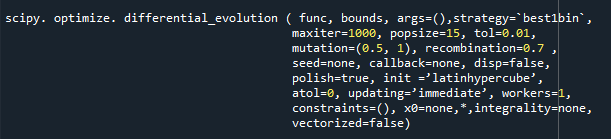
Let’s go over the function parameters:
The function must be callable with f(x,*args); bounds refers to the sequence of variables that can be specified in two ways: strategy is optional or a string with the default value “best1bin”; maxiter is optional or an int value; popsize is int or optional; tol is int or optional; mutation value is in float or optional; recombination value is in float or optional; the seed is none, int, NumPy, and Random.
In the next section, we will discuss a differential evolution function with the help of easy examples.
Example 1
Let’s begin with a straightforward example that will develop your interest in understanding the concept of differential evolution function. We used the differential_evolution() function to find the minimum value. But, to find the minimum value, the function required search bounds and a defined callable objective function. As a result, we define a function before using the differential_evolution function in the program. The reference code of the program is mentioned below:
from scipy import optimize
from scipy.optimize import differential_evolution
import matplotlib.pyplot as py
from matplotlib import cm
def func(p):
z,x=p
h = np.sqrt(z ** 4 + x ** 4)
return np.sqrt(h)
DE_bounds=[[-6,6],[-6,6]]
res=differential_evolution(func, DE_bounds)
print(res)
We imported libraries like SciPy and NumPy for array numerical calculations. We imported the differential_evolution function from the scipy.optimize module. Then, with the keyword “def”, we define the callable objective function and pass the parameter “p”. We successfully define the function that finds the square root of the NumPy variables addition, which is z, x. The square root value is stored in the variable “h”. We return the square root value in the defined function. It is returned as an argument.
After that, we settle the bounds of the variable that can be itemized by explaining the min and max values of the function. We execute the differential_evolution function with ‘DE_bounds”’ as an argument. We called the function value with a variable named res. In the end, we use the print statement to show the output. The result was displayed after running the program. The expected output screenshot is shown below:
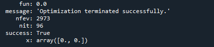
Differential_evolution() shows that the minimum value of the function is displayed at point (0, 0).
Example 2
This is another example of the differential evolution function. In this, we take arrays and apply different operations between them. The reference code of the program is mentioned below:
from scipy import optimize
from scipy.optimize import differential_evolution
def objective_func(d):
return ( d[1] - 1.2) / 2 + 0.5 * d[0] * 1.3 * (d[1]+0.5) ** 3
_bounds=[(-0.3,0.3),(-0.3,0.3)]
disp=differential_evolution(objective_func,_bounds,popsize=80,polish=False)
print(disp)
As shown in the previous screenshot, we successfully imported the SciPy.optimize.differential_evolution library and the NumPy library into the program. Now, we define an objective function on behalf of which we find a minimum value. We passed the mathematical expression in the objective function and returned a value as an argument to the defined function. The boundary between function values is a must. So, after defining the function, we fixed both the values (maximum and minimum).
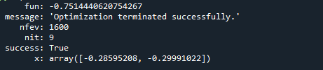
After defining all essential variables, we called the differential_evolution function to find the minimum value of a function. We saved the function’s minimum return value in a variable called disp. At the end of the program, we pass the disp variable in the print statement to display the result. After running the program, the minimum value of the defined function is displayed on the screen with bounds. The following is the output:
Example 3
As we can see, differential evolution returns different minimum values of an objective function based on its definition. Here, we take another example related to differential_evolution(). The reference code for this program is shown below:
from scipy import optimize
from scipy.optimize import differential_evolution
def obj_func(oper):
return 3 ** 9 / 0.2 + 6 /3 *2 ** 20
boundary=[(-0.5,0.5),(-0.5,0.5)]
out=differential_evolution(obj_func,boundary,polish=True)
print('Output is : ', out)
The libraries are successfully imported into this program because we cannot perform the operations we desire without them. As a result, we include the SciPy library in the program. After that, define the objective function with the required operation. We find the minimum value of that defined function. After adjusting the function’s boundary, we called the defined function in differential evolution to find the function’s minimum value. This is then kept in the variable. We display this by calling this variable in the print statement. The output of this program is shown below:
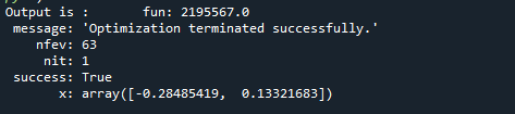
As in the previous screenshot, the minimum value of the function is [0.29236931, 0.16808904]. You can also run these examples in your environment to better understand the differential_evolution function concept.
Conclusion
Let’s take a quick recap of this article. We grasped the basic functionality of the differential evolution method that belongs to the SciPy library in Python. Python is the most recent language, with numerous flexible libraries. Most developers were aided in solving complex code structures by predefined functions and libraries. Differential evolution is a SciPy package optimization function or method used for minimization. When you use these previous examples in code, you more clearly understand the concept of differential evolution.
Source: linuxhint.com