“Scikit learn is the most widely used robust library that is being presented by Python. Scikit learn provides an efficient tool for Machine learning algorithms (supervised, unsupervised & reinforcement learning) and statistical modeling. Some major functionalities of sci-kit learn to include classification, regression, clustering, and Principal component analysis, i.e., dimensionality reduction. Scikit also deals with the support vector machines, gradient descents, and random forests (tree classifiers) that help achieve the results. Scikit learn is built on the most familiar libraries of python, such as Numpy, matplotlib, and scipy.”

Procedure

In this tutorial, we are going to learn about the Scikit learn library of python and how we can use this library to develop various machine learning algorithms. This guide will include the following contents that will be discussed one by one with a detailed explanation:

• Installation
• Graph plotting
• Various datasets and their utilities in Scikit learn
• Feature selection
• Training of a Machine learning model

Step 01: Installation

Before getting started with the scikit learn, we need to first install its package from the python repositories. To do this, we are required to have python (the latest version or any) downloaded and installed on our system. To download the Python on your system, navigate to the link i.e.

“https:// www. Python .org “. Once you’re redirected to this URL, go to Downloads and click on the python with any version you want to download as below:

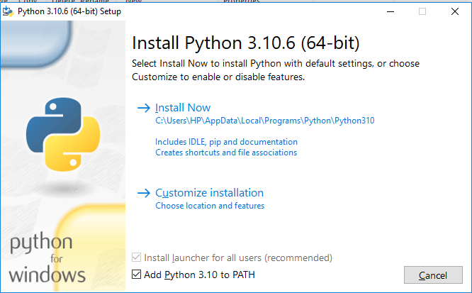
After the python is downloaded, we now need to install it. Select the customized installation option after adding the python to the path.

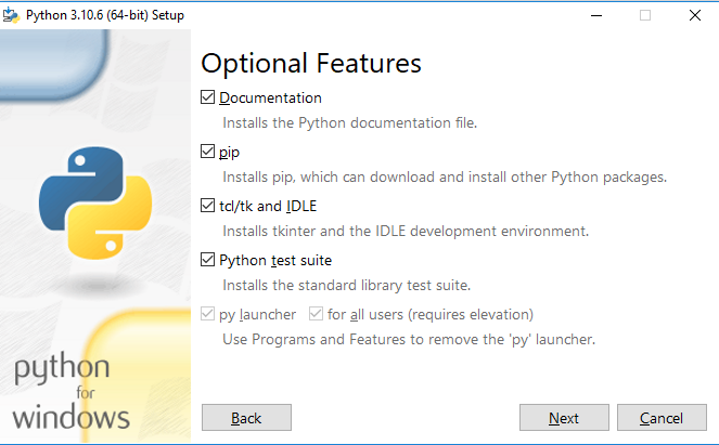
Check all the options on the popping window to install the packages of pip with python and continue and select next.

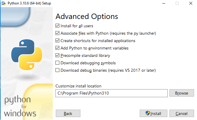
The next step will be to specify the location for the python packages, check all the given advanced options and specify the location and click on install; this will then begin the installation process that will continue for a while.

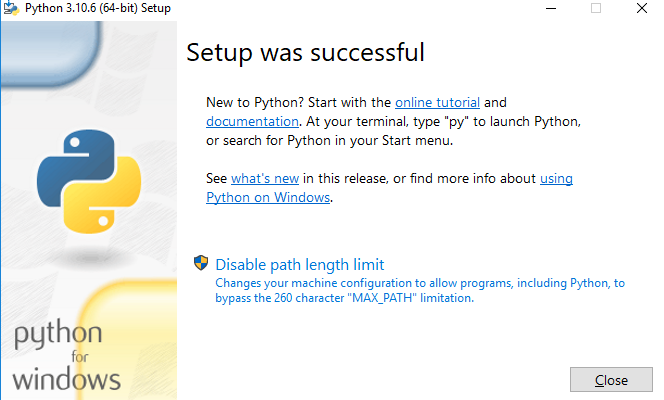
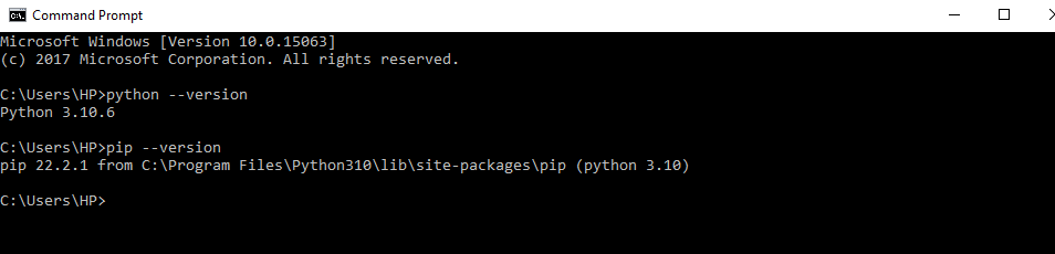
Now python is being installed on our systems. To open the Python shell type, put Python on the search menu and hit enter. The Python shell will then open. Now we’ll move forward to install the Scikit learn on python. For this, open the command prompt and type python to check if the python is running on the system or not. If the system returns the version of python, then this means that the python is running correctly. Then we need to check the version of pip so as to upgrade the pip packages:

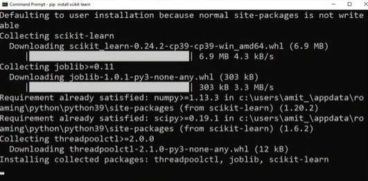
After checking both the python and pip versions, now type the following command on the command prompt to install the scikit learn on python.

After this, the scikit with all its packages will start to install.

Now Scikit learn has been installed in our system, and now we can use the scikit packages to develop any machine learning algorithm. After the successful installation of Scikit, we will now move forward to the next step, where we’ll get to know how to plot the graphs of the data using Scikit learn.

Step 02: Graph Plotting

Graphs are known as the visual tools that help to visualize the given information if the data in the data sets are too numerous or complicated enough to describe. Graphs emphasize representing the relationship between one or many variables. To work with the machine learning algorithms, we need to know the data representation for the analysis of data to train and test the data accordingly. Scikit learn provides many such visualization packages (in graphical form) for the various data sets.

Example# 01

The visualization of the data in the form of a graph can be obtained using the matplotlib package. Matplotlib is a python package that contributes as the base of the sci-kit learn plotting packages. Scikit learn integrates with the matplotlib for plotting (visual representation of the data or the results achieved after training & testing of the data in machine learning algorithms). Let’s try to implement an example using matplotlib.

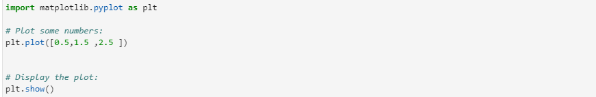
Suppose we want to plot some random numbers to visualize their relationship with each other. We can take these numbers at random, e.g., 0.5, 1.5, 2.5. To write the code, we’ll import the matplotlib library from the python packages as plt. After this step, we can now use plt instead of writing matplotlib in the entire code. Then using this plt, we will write a command to plot the numbers that we have already selected at random using the function “plt. plot (“selected numbers”)”. To display these numbers on the graph in the output, we’ll use the function “plt. show()”. The code can be created in a subsequent way:

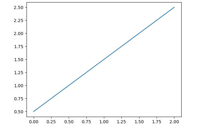
The numbers will then be displayed in the output on the graph:

Example# 02

If we want to plot the data in the form of a scatter plot, then we can use the function “scatter. plot ()”. The Scatter plot represents the data in the form of the dots data points. These plots work on two or more two variables. Each dot or data point on the graph represents the two different values (each on the x-axis and y-axis) corresponding to a data point in a dataset.

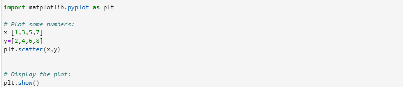
In the subsequent example, we’ll plot a scatter plot. To do so, we’ll import the matplotlib pyplot as plt. This plt can then be used in place of matplotlib. pyplot. After this, we’ll define the two variables x and y as x= 1, 3, 5, 7 and y = 2, 4, 6, 8. For the scatter plot, the dimension of x and y need to be matched. To plot both variables, we’ll use the function plt. scatter (“variable 1, variable 2”). To display these variables on the graph, use the function plt. show ().

The relationship between the two specified variables in the form of a scattered plot will then be displayed as:

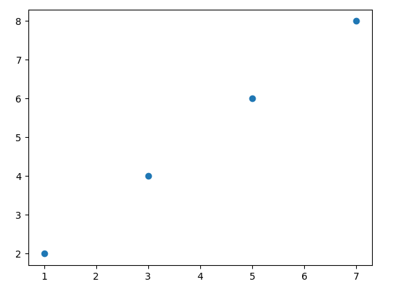
The above-mentioned examples can be used to plot the specific data and to know about their relationship with each other.

Example# 03

Now let’s suppose that we were working with some binary data set, and we have to classify the data as either belonging to class 0 or class 1. We developed a binary classifier for that data using a machine learning algorithm, and now we want to know how well this classifier is working. For this purpose, we may use an AUC-ROC_curve.

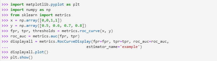
In AUC –RUC curve AUC tells which degree the classifier developed can predict the classes correctly, either as 0 or 1, and ROC depicts the probability of the classifiers depicting the classes correctly. AUC-RUC_ curve displays the curve between fpr (y-axis) and tpr (x-axis), which are both nd-arrays. To implement this AUC-RUC curve, first, import the matplotlibpyplot as plt so that we can call plt for plotting.

Then we’ll import the numpy as np to create the nd-arrays. After this import from sklearn metrics. Now we will specify the x and y by using the np. array () to create the nd-arrays. Nd-arrays use the Numpy to store the sequential numbers in them. To specify the fpr and tpr and thresholds, we’ll use the method “metrics.roc_curve (x, y)” and then we’ll use these values of fpr and tpr to store in the roc_auc by calling the function “metrics.auc ()”.

After these values are specified, we’ll call the function using “metrics. RocCurveDisplay ()” by passing fpr, tpr, and roc_auc in its arguments and storing them in variable display all. Then we’ll call the function. plot () and plt. show () to display the ROC-AUC curve with the specified parameters in the output as follows:

After running the above-mentioned code, we get the following output:

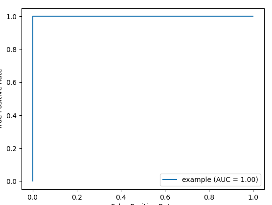
The RUC-AUC curve has been displayed in the output now, which represents how much our developed classifier has predicted the classes as 1 or 0 correctly. ROC-AUC curve works for the datasets with binary classification.

Example # 04

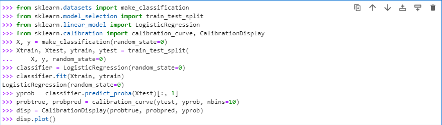
Another graph plotting method using the scikit learn the calibration curve. The calibration curve has another name: the reliability diagram; this curve plots the average of predicted probability against the positive class at the y-axis of the curve by taking the input from the binary classification classifier. To implement this calibration curve, let’s solve an example where we will first import the data set “make classification” from the sklearn datasets package, then import train and test split from sklearn model selection, then using the sklearn linear model selection import logistic regression and after that import calibration curve and display from the “sklearn calibrations”.

Once we have imported all important and required packages, now load the “make classification” using the load “dataset_name ()” method, after this we will split the data for train and test purposes using the “train_test__split ()” method, then we will build the classification model using “logisticregression ()” and fit this model on x_train and y_train.

Now by using the labels and probabilities that have been predicted using “classifier. predict probability ()” bypassing the xtest as its input argument, call the method “calibration curve () “to plot the calibration curve first and then display it using “Displaycurve ()”.

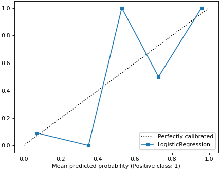
The output displays the plotting of the calibration curve that has used the true predicted probabilities from a binary classifier.

Step 03: Various Datasets and Their Utilities in Scikit Learn

To work with machine learning algorithms, we need to have the datasets that we can use to build the specific algorithms on and achieve the desired outputs. Scikit learn comes with some packages that have default embedded datasets stored in it by the name sklearn. datasets. To work on the data sets, we can either read them using sklearn default datasets repositories or by generating them.

The datasets that sklearn provides its user are some relatively small toy datasets and other real-world data sets that are huge and have information related to worldly applications. The standard size and small datasets can be obtained using the dataset loaders, whereas the real-world datasets are loaded through data set fetchers.

In this example, we’ll first import the toy data sets from “sklearn. datasets”. To import the data set, we’ll use sklearn.datasets. Sklearn.datasets allow importing the datasets from its default datasets. Different datasets can be loaded from sklearn.datasets using this command.

Here we have imported the digits’ dataset from the Sklearn.datasets. We can load any other dataset using the same command with the simple modification; that is, we have to replace the “load_digits” with the name of that specific data set that we want to load in the above-mentioned command. Now in the next step, we will load the dataset using the method “data set_name ()” and then store it in any variable, let’s say dataset, as we’ve done in this command

Till this step, the data set has been downloaded in the digits. To display the data in this dataset, we’ll use the print function and will pass the variable name.data in the arguments of the print function.

Now we’ll run these all above explicitly mentioned commands in the form of a code, and it will give the output as:

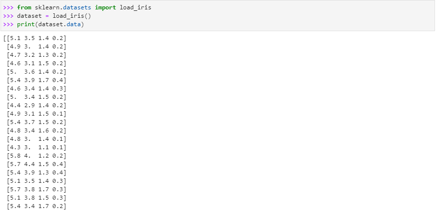
After executing the code, we got an output that displays all the data that is stored in the data set of load _digits.

If we want to know about the specification of the dataset in terms of how many classes are there in the data set or how many features are there for the dataset plus the sample size of the dataset, that is, how many examples have been given for each dataset.

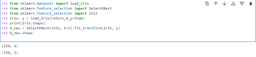
To get this information, we can simply use the function “dataset_varaiable name. shape”. To implement this, import the data set (load_iris ) from sklearn.datasets and then load this dataset by calling the method “load_iris ()” and storing it in “iris. load”. Then print the specification of the data set using the print ( loadiris.shape ) in the following way:

The above code would have the following output after execution:

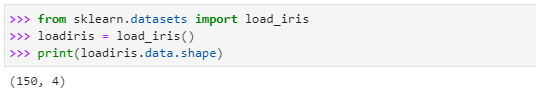
The output has returned the values (150, 4). This means that the data set has 150 sample examples and 4 attributes that we can use to create our machine learning algorithm according to the demand.

In the next example, we’ll now learn how to import real-world datasets and work on them. For real-world data, we fetch the files using the fetching function that downloads and extracts the dataset from the specific website’s cache/archive and loads it in the sklearn. datasets.

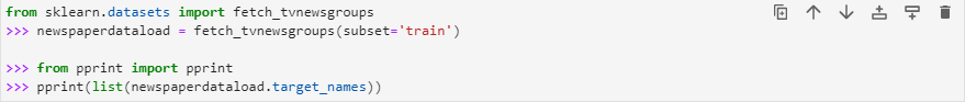
Let’s take real-world data from the real-world datasets using the sklearn.datasets and work on it. Here we would like to take the data from some newsgroup websites, “tv newsgroups websites”. Now we will import the dataset for this specific website by first fetching the files from the website’s repository. Then we will load the training data from the fetched files of this data to the sklearn.datasets calling the loading method, i.e., “dataset_name (subset=” either test or train data to be entered”)” and then will store it in some variable “newspaperdataload”.

After this, we will simply display the dataset’s target names. “Target names” are the files that contain the real data files of the datasets. Let’s call the print function to display the names of the files present in the data set by writing the commands:

We have imported the pprint here because the target name contains the list of the file, and we want this list to be displayed as it is. To display this list, we have imported the pprint package first, and then using it, we have displayed the list of the file names in the dataset that we have already loaded in “sklearn.datasets” by fetching the files from the website. We have implemented the above-mentioned code in python, and its output came out to be like this:

Now the list of the datasets has been displayed by the system. If we want to know the attributes of this dataset, e.g., the number of sample examples the data set contains, the total number of features in the data set, etc. We can simply use the print (dataset_name. filename. shape) since, as we have already explained that all the information of the dataset is stored in the file_name or target_name file, and it will return the attribute information of the dataset as it is.

Step 04: Feature Selection

In machine learning algorithms, the most important aspect that controls the output of the algorithm is the features. Features contribute majorly to building any machine learning algorithm. All the processing is done on the data sets that are based on the features. Features may make the algorithms robust or a complete failure in terms of accuracy (best prediction or estimation) for the decision boundary. If there exist redundant features or a greater number of features that are required, then this contributes to overfitting in the output.

Overfitting is the phenomenon in which a model that is trained on data sets having more features than required and has a training error closest to zero, but when it is trained on the testing data set, the model does not work well on that test data set and hence fails to make the correct decisions. To avoid the chances of the trained model being overfitted, we drop some of the unnecessary features. This dimensionality reduction can be made in several ways using the scikit learn.

Example #01

The first method to remove the feature is through a low variance threshold; in this type of feature selection, we remove those features from the datasets having low variance that are below the given thresholds. Low variance features are those that contribute the same value throughout the data set.

Let’s try an example for feature reduction. Suppose that we have a dataset that has three features in binary data. In our example, the digit datasets have four columns as their four features. If we want to remove one feature with all its sample examples from the dataset, then we will use the variance formula and build a variance threshold on that. If any feature has low variance, then the threshold will be then removed from the dataset.

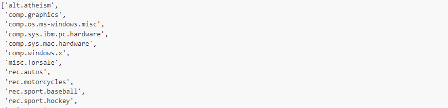
We’ll first import the variance threshold from the “sklearn feature_selection”. Once the variance threshold is imported, we’ll then set the value of this threshold which, in our case, we have defined as “0.5”. So, any feature columns that have a value less than this threshold will drop out of this digit data set.

To do so, we will call the method “variance threshold ()”. In the arguments of the function, we will pass the threshold value to be 0.5 and store it in some variable “thresholder”. After this, we will call the function “thresholder. fit_transform ()” and pass the dataset to this function and let it store it with the name new_dataset. Once we are done with these steps, we’ll print the data set as shown:

As it can be seen in the output that before we applied the variance threshold to the dataset, it had 4 features, and now after the application of the variance threshold on the dataset, we instructed the system to remove all the columns having variance below the threshold value, i.e., 0.5, the output displays three columns in the dataset which means that the one column was calculated to have variance less than the threshold, so it was dropped out of the dataset to avoid the redundancy in the dataset and to make the model trained on the data set to be more precise in terms of accuracy and avoiding overfitting.

Example #02

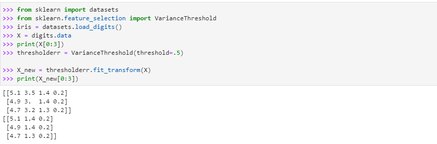
The second method to select the features in the dataset is given by the “select k-best” method. For the implementation of this method, the iris dataset will be imported from the “sklearndatasets,” and then we will load this data set and save it in some random variable such as iris. Then to load the dataset, we will call “loaddataset_name ()”.

Chi2 measures the difference between expected and observed features and is used for classification tasks. After loading the dataset into iris and importing the select k best and chi2, we will now use them in the “fit. transform() function”. The selectkbest (chi2, k = 2). fit.transform (), it first fits the data taking the training data as input and then transforming it. Then the k in the selectKbest method drops the columns and selects those features that have scored the highest in features. In our case, we will select the two features as we select the k value equal to 2.

In this example, when we simply loaded the data set and then displayed it, there were four columns as features in the dataset, but now after we have applied the selectKbest method with k=2 on the dataset now, the new dataset came out having two columns as features this means that the selectKbest has selected the two best features from the original dataset.

Example #03

Another way to select the important feature from the data set is given by scikit learn using the “Recursive Feature Elimination (RFE)”. RFE drops the less important features from the data set by doing the recursive training of the dataset. RFE selects the feature number for itself by using the median of the total number of features in the dataset, and it drops only one feature from the dataset at every iteration. To implement RFE, first import the libraries that are required to build the code through these commands.

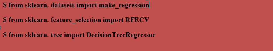
Now we have successfully imported the packages for RFE from sklearn. feature. selection. To create the dataset, we have loaded the “make_regression ()” function, and in its arguments, we have passed those parameters that we want in the data set.

Then we print this dataset to know about the exact shape or attributes of the dataset. After displaying the dataset, we will now use the Recursive Feature eliminator. For this purpose, we will make a model as decisiontreeRegressor (). After the model is completed now using the RFECV () that we imported earlier, we will pass the verbose, model/estimator, step, scoring, and cv as the parameters being required in the arguments of RFECV.

Now to remove the recursive feature, we will fit and transform the data. The whole explained procedure can be written as the code below:

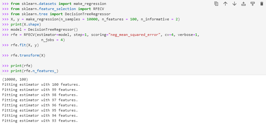
Now the features will be recursively dropped according to our requirement after every iteration, as it can be clearly shown in the output. This recursive feature elimination will be continued till we reach the point where we are left with two important features out of the total 100 features present in the original dataset.

Example #04

Another method that we can use to remove the extra features, or we can simply drop them due to their redundancy, is the “Selectfrom Model” along with the “linear models”. When the theses linear models are somehow penalized with the l1 norm, their solution exists sparsely since most of their coefficients become equal to zero.

In dimensionality reduction or feature selection, these linear models, along with the selectfrom model, help to select that non-zero co-efficient. They work mostly for the regression problem. To implement the selectfrom model, we need to first import the linearSVC from sklearn.svm, LinearSVC is the linear support vector classifier that finds the best fit line (hyper-plane) to divide and classify the data in different categories; once we get the hyperplane in lsvc, we can then provide any feature to this best fit model to know which class that feature would belong to, then we will import the data set from the sklearn. ata sets, and after this, we will have to import the “selectfrom model” from sklearn.feature selection.

After the required packages have been imported, we load the iris data set using load_dataset () and then display the attributes of the iris data set in terms of sample examples and the number of features it has using the “ .shape” method. After knowing the shape of the data set, we will now apply the “linearSVC ().fit(_loaded data set )” model with C=0.01, a penalty of the linearsvc = l1 as its input argument. Then build the model using “selectfrom model()” and then transform the model using “model.transform()”. Now display the new transform data set and show its attribute using the data “set_new.shape”.

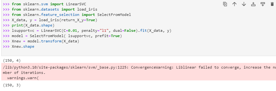
The shape of the data set before applying the “selectfrom model” for the feature selection was (150, 4), which means that it had 150 sample examples and four attributes, but once we applied the feature selection on the data set using “linearSVC” and Selectfrom model the shape of data set has been transformed to (150, 3) which means that the one feature has been dropped out from the data set.

Step 05: Data Preprocessing

The data sets that we work with to develop and train different machine learning algorithms on them are not always the ones in their perfect form to use for building the model. We must modify these data sets according to our requirements. The very first step we need to do after loading the dataset and before training the model is data pre-processing. By pre-processing of data, we mean:

• Feature scaling
• Feature normalization / standardization

Feature Scaling

The most important task in data pre-processing is feature scaling. Feature scaling is done to make all the features of the data set have the same unit; otherwise, the algorithm will not train properly, and it can affect the performance of the algorithm by slowing down the process. The scaling can be done using the minmaxscaler or maxabsscaler. Feature scaling sets the feature values’ ranges between zero and one mostly, and sometimes on demand, it can limit the value of a feature to its unit size.

Here we will implement an example in which first we are going to import preprocessing from sklearn, and then we will import numpy. Numpy is used in the functions where we need to work with arrays. Now we’ll create an nd-array using numpy. To do feature scaling on this array that we have created, first, we will use the method “preprocessing. MinMaxScaler()”. After this step, we apply the minmaxscaler to the array by calling the method “minmaxscaler. fit_transform()” and will pass this array in its arguments. The code can be re-written as:

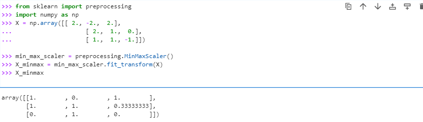
The output after the feature scaling has been performed on the “x” gives the value of an array between zero and one. The maxabsscaler works mostly the same as the minmaxscaler, but this scaler scales the data values range between negative one ( -1 ) and positive one ( +1). The code for the MAXabsScaler is given by:

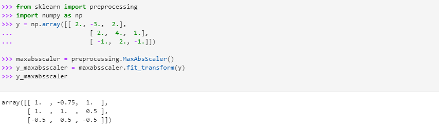
In the output, the values of data “x” have been returned in the continuous form from the range varying between -1 to +1.

Feature Normalization / Standardization

We will learn about the data pre-processing techniques in this example. Let’s first import from sklearn preprocessing and after importing the preprocessing from sklearn, then also import numpy since we are now going to work with nd arrays. Now create an nd-array and store it in “X”. Now we need to perform the mean normalization/standardization on this data. To do this, we will use the conventional method “preprocessing. standardscaler. fit (“type here the data to be normalized”)”. The value from the function will then be saved in a variable, e.g., scaler. Now perform the standardization on the given data X with method, e.g. “scaler. transform (“data”)” and display the newly transformed data then:

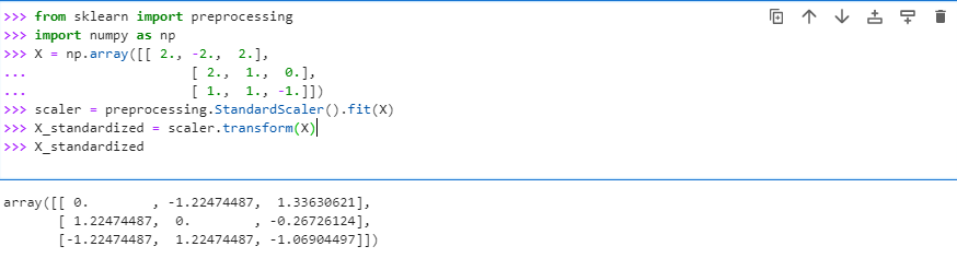
The data “x” has been standardized with the mean value closest to zero. Normalization/standardization of the data is done to avoid any redundant or duplicates in the data set. Mean normalization/ standardization ensures keeping only the related data in the data sets. Moreover, it also deals with any problems caused due to modifications, e.g., deletion of data, the addition of new data, or any update in the data sets that might become a hurdle in the future.

Now that we have learned most about the scikit learn packages that we can use to build the machine learning algorithms. We should test our abilities with the scikit learn a function that we have used above in this guide and develop a machine learning algorithm to first train a model on the specific data set and then test that model by running it on the unknown test data set to gain a hands-on experience on this scikit learn functions/packages. Let’s kick off the implementation of the scikit learn functions for the machine learning algorithm or model.

Step 06: Model Training Using Scikit Learn

We will train the “linear regression model” on the house pricing data set that we will create ourselves in the code later. Linear regression finds the best line fit for the data points given in the data set. This line is plotted on the data points on the graph. We use this line then to predict the values that our train model will predict when it will be tested on some test data with the belief that output data points generated after running the test data on the model would follow the line as the original data or training data has followed.

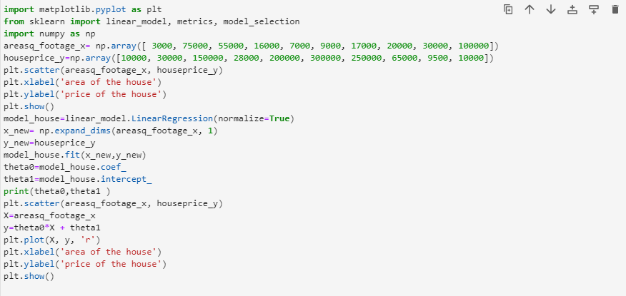
To work with the linear regression model, we need to import the matplotlib library, then from scikit learn, we will import the linear model, matrices, and any model selection to train the model later in the code. To create the data set of house price, we will import np from numpy and create the two nd-array with names “areasq_footage_x” and “houseprice_y,” respectively.

After creating these two nd-arrays, we will plot their values on the plot using the “scatter.plot()” by labeling the x-axis of the graph as the ‘area of the house ‘and the y-axis as the ‘price of the house ‘. Once the data points have been plotted, we will then train the model using the “linearRegression () model”. We will then expand the dimensions of the nd-array “areasq_footage_x,” and then it will be stored in the new variable “x_new”. Then we’ll use the “model_house.fit ()” and will pass the “x_new” and “houseprice_y” in its input arguments to fit the model for the best line.

We will create the hypothesis of the best line fit by “y = theta0* X + theta1” and will plot these expected outputs to the real given data and plot the graph. This graph will let us know the best fit line for the given data points, based on which we will predict the output of the data points of test data predicted as correct or not.

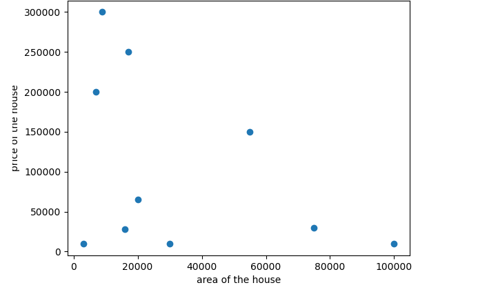
This is the graph we obtained before training the model. All the data points here have been plotted following the values of both the x-axis and y-axis.

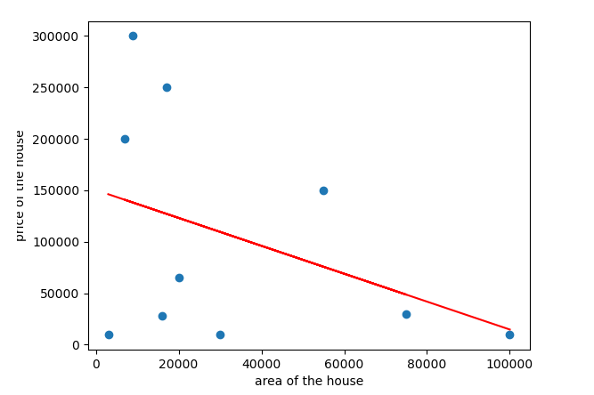
This graph is the output of the trained model, and it shows the best fit line to predict the output for the data points if the trained model is evaluated on some test data.

Conclusion

Scikit learn is a library for python that uses the sklearn package to work with its different available functions for building any machine learning algorithm. In this tutorial, we have learned scikit learn from very basic steps (Installation of the scikit learn on python to the complex training a model using the scikit learn packages). In between from the basic to the complex level, we have discussed graph plotting, loading datasets, feature selection, and data pre-processing. We hope you will find this tutorial helpful in developing your knowledge regarding Sci-kit learn.