Before starting our topic, let us understand what the moving average is. In statistics, a moving average is a technique to calculate and analyze data points. It calculates data points by making a series of an average of different subsets from a full dataset. So, a moving average is a measurement that catches the typical change in an information series over time. Moving is one of the most flexible and frequently used technical analysis indicators. Since it is so simple to use, professional investors employ it as a means of a certain set of data in statistics. We can also calculate a moving average in a shorter period by using it on daily or minute data.For example: When determining a 10-day moving average, in our instance, we will just sum up the closing prices from either of the previous ten days and divide the result by ten. On the next day, we will also calculate the price in the last ten days which means we will not be calculating the price of the first day. It will rather be replaced by our price yesterday. The data changes in this manner with every moving day, it is known as the moving average for this reason. The purpose of the moving average is to determine the start of a trend, then follow its progress and also report its reversal in case it occurs. The formula to calculate the moving average is Ft = (Dt1+Dt2+Dt3…+Dtn)/n. Where Dt is Demand in period t and Ft is Forecast in time t.

Syntax:

We can calculate the moving average in various ways which are as follows:

Method 1:

It returns the sum of elements in the given array. We can calculate the moving average by dividing the output of cumsum() by the size of the array.

Method 2:

It has the following parameters.

a: data in array form that is to be averaged.

axis: its data type is int and it is an optional parameter.

weight: it is also an array and optional parameter. It can be of the same shape as a 1-D shape. In the case of one dimensional, it must have an equal length as that of “a” array.

Note that there seems to be no standard function in NumPy to calculate the moving average so it can be done by some other methods.

Method 3:

Another method that can be used to calculate the moving average is:

In this syntax, a is the first input dimensional and v is the second input dimensional value. Mode is the optional value, it can be full, same, and valid.

Example # 01:

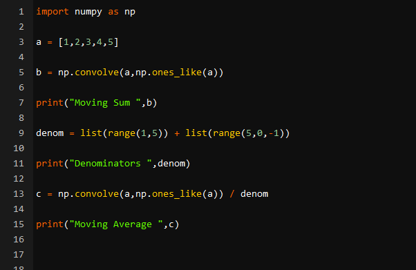
Now, to explain more about the moving average in Numpy let us give an example. In this example, we will take out the moving average of an array with the convolve function of NumPy. So, we will take an array “a” with 1,2,3,4,5 as its elements. Now, we will call the np.convolve function and store its output in our “b” variable. After that, we will print the value of our variable “b”. This function will calculate the moving sum of our input array. We will print the output to see whether our output is correct or not.

After that, we will convert our output to the moving average using the same convolve method. To calculate the moving average, we will just have to divide the moving sum by the number of samples. But the main problem here is that as this is a moving average the number of samples keeps changing depending upon the location that we are at. So, to resolve that issue, we will simply create a list of the denominators and we need to turn this into an average.

For that purpose, we have initialized another variable “denom” for the denominator. It is simple for list comprehension using the range trick. Our array has five different elements so the number of samples in each place will go from one to five and then back down from five to one. So, we will simply add two lists together and we will store them in our “denom” parameter. Now, we will print this variable to check whether the system has given us the true denominators or not. After that, we will divide our moving sum with the denominators and print it by storing the output in the “c” variable. Let us execute our code to check the results.

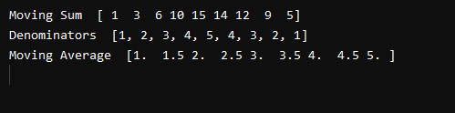
After the successful execution of our code, we will get the following output. In the first line, we have printed the “Moving Sum”. We can see that we have “1” at the start and “5” at the end of the array, just like we had in our original array. The rest of the numbers are the sums of different elements of our array.

For example, six on the third index of the array comes from adding 1,2, and 3 from our input array. Ten on the fourth index comes from 1,2,3 and 4. Fifteen comes from summing up all the numbers together, and so on. Now, in the second line of our output, we have printed the denominators of our array.

From our output, we can see that all the denominators are exact, which means that we can divide them with our moving sum array. Now, move to the last line of the output. In the last line, we can see that the first element of our Moving average Array is 1. The average of 1 is 1 so our first element is correct. The average of 1+2/2 will be 1.5. We can see that the second element of our output array is 1.5 so the second average is also correct. The average of 1,2,3 will be 6/3=2. It also makes our output correct. So, from the output, we can say that we have successfully calculated the moving average of an array.

Conclusion

In this guide, we learned about moving averages: what moving average is, what is its uses, and how to calculate the moving average. We studied it in detail from both mathematical and programming points of view. In NumPy, there is no specific function or process to calculate the moving average. But there are different other functions with the help of which we can calculate the moving average. We did an example to calculate the moving average and described every step of our example. Moving averages is a useful approach to forecasting future results with the help of existing data.