In data science and Statistics, it is a regression model if the dependent variable results in categorical values like True/False, Yes/No, or 0/1. Usually, the logistic regression model is binomial. However, it can be extended. It measures the probability of the successfulness or failure of an event as a dependent variable which is based on a mathematical equation. This equation relates the dependent variable (response variable) with the independent variables (predictor).

We can say that logistic regression is a generalized form of linear regression but the main difference is in the predicted value range is (-∞, ∞) while the range of predicted value in logistic regression is (0,1). In this post, we will learn about logistic regression and how to implement it in the R programming language. 

Why use logistic regression

After understanding the relationship between independent (predictor variables) and dependent (response variable), linear regression is often used. When the dependent variable is categorical, it is better to choose logistic regression. It is one of the simplest models but very useful in different applications because it is easy to interpret and fast in implementation.

In logistic regression, we try to categorize the data/observation into distinct classes which shows that logistic regression is a classification algorithm. Logistic regression can be useful in different applications such as:

We can use the credit record and bank balance of a customer to predict whether the customer is eligible to take the loan from the bank or not (response variable will be “eligible” or “non-eligible. You can access from the condition above that the response variable can have only two values. Whereas in linear regression the dependent variable can take more continuous multiple values.

Logistic regression in R in Ubuntu 20.04

In R when the response variable is binary, the best to predict a value of an event is to use the logistic regression model. This model uses a method to find the following equation:

Xj is the jth predictor variable and βj is the coefficient estimate for the Xj. An equation is used by the logistic regression model to calculate the probability and generates the observation/output of value 1. That means the output with a probability equal to 0.5 or greater will be considered as value 1. Other than that all values will be considered as 0.

The following step-by-step example will teach you how to use logistic regression in R.

Step 1: Load the data for the model in R
First, we have to load a default dataset to demonstrate the use of the model. This dataset consists of 1000 observations as displayed below.

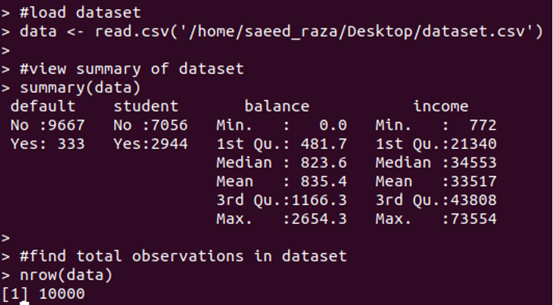
In this dataset columns, the default is showing whether an individual is a default. The student is showing whether an individual is a student. Balance is showing the average balance of an individual. And income is indicating the income of an individual. To build a regression model the status, bank balance, and income will be used to predict the probability of the individuals are default.

Step 2: Training and test samples creation
We will divide the dataset into a testing set and a training set to test and train the model.

70% of data is used for the training set and 30% for the testing set.

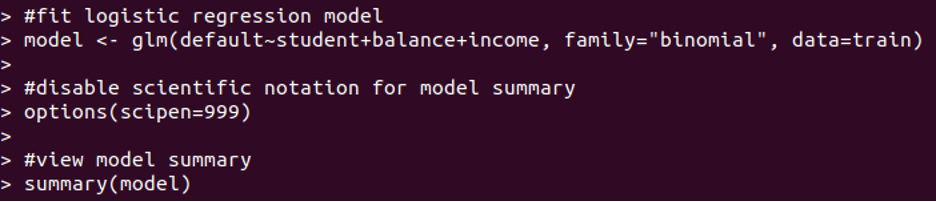
Step 3: Fitting Logistic regression
In R, to fit logistic regression we have to use a glm function and set the family to binomial.

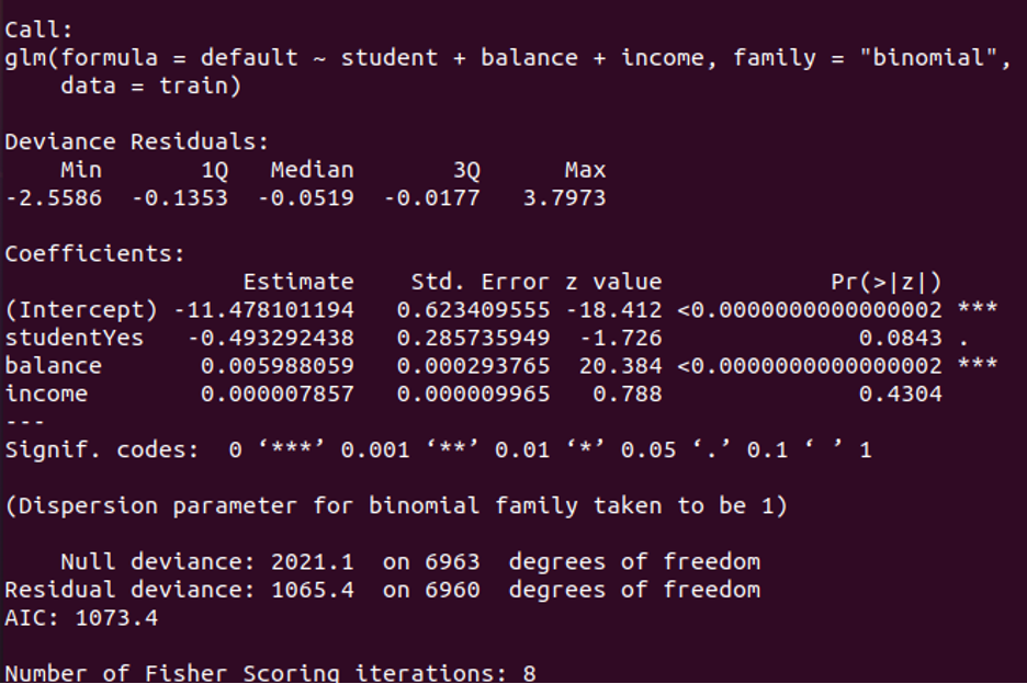
In log odds, the average change is indicated by the coefficients. The P-value of student status is 0.0843 P-value of balance is <0.0000, P-value of income is 0.4304. These values are showing how effectively each independent variable is at predicting the likelihood of default.

In R, to check how well our logistic model fits in data McFadden’s, R2 metric is used. It ranges from 0 to 1. If the value is close to 0 it indicates the model is not fit. However, values over 0.40 are considered a fit model. The pR2 function can be used to compute McFadden’s R2.

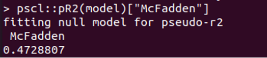
As the value above is above 0.472, it is indicating that our model has high predictive power as well as the model is fit.

The importance of a function can also be calculated by the use of the varImp function. The higher value indicates that the importance of that variable will be higher than others. 

Step 4: Use the Logistic regression model to make predictions
After fitting the regression model, we can’t make predictions about whether an individual will default or not on different values of balance, income, and the status of the student:

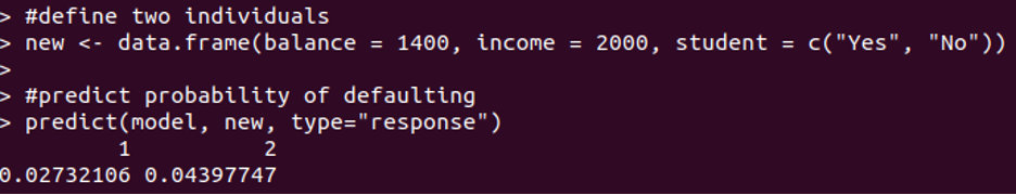
As we can see, if the balance is 1400, income is 2000 with the status of student “Yes” having a 0.02732106 probability of defaulting. On the other hand, an individual having the same parameters but Student status “No” has a 0.0439 probability of defaulting.

to calculate every individual in our dataset, the following code is used.

Step 5: Diagnosing the Logistic regression model:
In this last step, we will analyze the performance of our model on the test database. By default, the individuals having a probability greater than 0.5 will be predicted “default”. However, using the optimalCutoff() function will maximize the precision of our model.

As we can see above, 0.5451712 is the optimal probability cutoff. So, an individual having a probability of 0.5451712 of being “default” or greater will be considered as “default”. However, an individual has a probability less than 0.5451712 will be considered as “not default”

Conclusion

After going through this tutorial you should be familiar with logistic regression in R programming language in Ubuntu 20.04. You will also be able to identify when you should use this model and why it is important with binomial values. With the help of codes and equations, we have implemented the five steps of using the logistic regression in R with examples to explain it in detail. These steps cover everything starting from loading data to R, training and testing the dataset, fitting the model, and prediction making to model diagnostics.