LibreOffice Calc Basics VIII: HLOOKUP
This tutorial explains the horizontal variant of vlookup formula, called HLOOKUP, on LibreOffice Calc. We will learn first about data transposing, then manipulating it with the formula. As a reminder, if you haven't followed this LibreOffice Calc series, read the first and second parts here. Now let's try.
![]()
Subscribe to UbuntuBuzz Telegram Channel to get article updates.
Dataset
To create the dataset, you will learn about Transpose, a technique to turn rows into columns and vice versa in a data table. With this, a vertically stacked data will be horizontal -- thus we will need HLOOKUP for it.
Before:
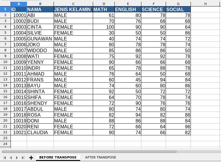
the data is stacked vertically, spanning across A1:G22,
while the scores span across D2:G22)
After:

(The same dataset, transposed,
and now it is put horizontally, spanning across A1:V7
while the scores span across B2:V7,
will be used in HLOOKUP formula)
To make this dataset:
1. Prepare the previous dataset from Calc Basics VII.
2. Copy the dataset.
3. Create a new spreadsheet document.
4. Right-click at A1.
5. Paste Special > Transpose.
6. Save as calc-08-hlookup.ods.
Dataset created.
Creating Drop Down Menu
Similar to doing VLOOKUP, we need a drop down once again in this exercise:
1. Put cursor at B9
2. Go to menu Data > Validity > Allow: Cell Range > type Source: $Sheet1.$B$2:$V$2 > OK.
Alternatively, click select and drag cells horizontally from ABI to CLAUDIA as input to Source. See animation below.
3. Drop down menu created at B9.
4. Try to click the drop down button and you should be able to select from ABI to CLAUDIA.

(Animation: showing how to create a drop down menu)
HLOOKUP
0. Select ABI from the student selector.
1. Put cursor after math score cell or B10.
2. Type the formula =HLOOKUP(B9; B2:V7; 3; 0)
3. You get his math score by 61.
4. Repeat step 1-3 for English score with =HLOOKUP(B9; B2:V7; 4; 0)
5. You get his English score by 80.
6. Repeat step 1-3 for Science score with =HLOOKUP(B9; B2:V7; 5; 0)
7. You get his Science score by 78.
8. Repeat step 1-3 after Social score with =HLOOKUP(B9; B2:V7; 6; 0)
9. You get his Social score by 78.
10. Switch ABI to CLAUDIA and other students one by one. You should get individual student's scores correctly.

(HLOOKUP formula for individual scores,
notice the similarity and the only difference is
the row numbers from 3 to 6)
Split View
Because doing HLOOKUP might lead to a very long horizontal data, you can enable menu View > Split View > adjust the lines and area to simplify how the data look. See next picture for example.
Final Result
Below is an example of three results of HLOOKUP against SILVIE, SHINTA, and DONI to show his/her score individually. You can evaluate the scores match the table. See picture below.
Also note the new skill you acquired, Split View, a helpful one that allows you to simply cut the long data to show only the important ones by adjusting the partitions and horizontal scrollbar. In the picture below, it is depicted as a thick, vertical grey line. Notice the number 10006 goes straight to 10013.

(Horizontal data with four HLOOKUP tests in split view,
notice SILVIE's, SHINTA's, and DONI's scores)
To this point, you have finished all 14 basic Calc formulas which are most frequently used in jobs from SUM to VLOOKUP. Also remember that these all are compatible with Microsoft Excel's. Finally, see you in our future LibreOffice series.
Source: Ubuntu Buzz !