Grid Search with MLflow
Benefits of Grid Search
- Automated Hyperparameter Tuning: Grid search automates hyperparameter tuning which allows the systematic exploration without manual trial and error.
- Reproducibility: Grid search ensures test validity by reproducibly obtaining the reproducible outcomes which enhances communication and reliability.
- Exhaustive Search: GS efficiently finds optimal hyperparameters for a model by exhaustively searching combinations.
- Robustness: Grid search is a robust technique that is resistant to data noise which reduces overfitting.
- Simple to use: Grid search is simple to use and comprehend which makes it a viable method for hyperparameter tuning.
- Model Comparisons: Grid search simplifies the model comparison and evaluation metrics selection.
Drawbacks of Grid Search
- Computational cost: Grid search is computationally expensive for tuning a large number of hyperparameters.
- Time-consuming: It is time-consuming for complex hyperparameter adjustments.
- Not always necessary: It is now always required; random search is the best alternative to it.
Example: Finding the Best Model Settings for University Admission System
Let’s look at a grid search example for hyperparameter tuning inside the framework of an online university admissions system. In this example, we use the scikit-learn and a straightforward Gradient Boosting Classifier (GBC) classifier to forecast a student’s likelihood of being accepted to a university based on factors like GPA points, SAT scores, ACT scores, and extra-curricular activities. Multiple options are available for grid search instead of GBC including Logistic Regression (LR), SVM (Support Vector Machine), etc.
Generate a Random Data for Online Admission System Using MLflow for Grid Search
Python’s Pandas and random packages can be used to create a fictitious dataset for the admissions system. With random values for the APP_NO, GPA, SAT Score, ACT Score, Extracurricular Activities, and Admission Status columns, this code generates a synthetic admission dataset. The num_students variable controls how many rows are there in the dataset.
The admission status is randomly set based on a 70% acceptance rate, and the random module is used to produce random values for several columns. For demonstration purposes, the following code piece creates a fake admission dataset with random values and is saved to the std_admission_dataset.csv file:
Code Snippet:
import pandas as panda_obj
import random as random_obj
# Set the number of records for the student dataset to generate
students_records = 1000
# Create lists to store data
std_application_numbers = ['APP-' + str(random_obj.randint(1000, 9999)) for _ in range(students_records)]
std_gpa = [round(random_obj.uniform(2.5, 4.0), 2) for _ in range(students_records)]
std_sat_scores = [random_obj.randint(900, 1600) for _ in range(students_records)]
std_act_scores = [random_obj.randint(20, 36) for _ in range(students_records)]
std_extra_curriculars = [random_obj.choice(['Yes', 'No']) for _ in range(students_records)]
# Calculate admission status based on random acceptance rate
std_admission_status = [1 if random_obj.random() < 0.7 else 0 for _ in range(students_records)]
# Create a dictionary to hold the student data
std_data = {
'APPLICATION_NO' : std_application_numbers,
'GPA': std_gpa,
'SAT_Score': std_sat_scores,
'ACT_Score': std_act_scores,
'Extracurricular_Activities': std_extra_curriculars,
'Admission_Status': std_admission_status
}
# Create a DataFrame DataFrame_Student from the dictionary
DataFrame_Student = panda_obj.DataFrame(std_data)
# Save the DataFrame DataFrame_Student to a CSV file named std_admission_dataset.csv
DataFrame_Student.to_csv('std_admission_dataset.csv', index=False)
print("Student Data Successfully Export to CSV File!")
Code Execution:
Use the Python command to compile the code, then use the pip command to install a specific module if you encounter a module error. Use the pip3 install command to install the given library if Python is version 3.X or higher.
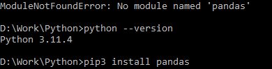
Successful Execution:
![]()

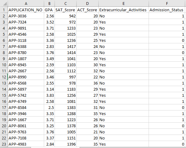
Sample Data Screenshot:
Step 1: Import the Libraries
- The MLflow library for machine learning experiment tracking
- The Pandas library for handling the data processing and analysis, as well as the mlflow.sklearn package for integrating the Scikit-Learn models
- The fourth line imports the “warnings” library to suppress the errors
- The ParameterGrid class for grid search in sklearn.model_selection module
- GridSearchCV and GradientBoostingClassifier from sklearn.model_selection and ensemble, respectively, for grid search and gradient boosting classifier models
- The accuracy_score and classification_report functions from the sklearn.metrics module to calculate the model accuracy and generate classification reports
- The code imports the OS module and sets the GIT_PYTHON_REFRESH environment variable to quiet.
Code Snippet:
import mlflow
import mlflow.sklearn
import warnings as warn
import pandas as panda_obj
from sklearn.model_selection import train_test_split as tts, ParameterGrid as pg, GridSearchCV as gscv
import os
from sklearn.ensemble import GradientBoostingClassifier as GBC
from sklearn.metrics import accuracy_score as acs, classification_report as cr
os.environ["GIT_PYTHON_REFRESH"] = "quiet"
Step 2: Set the Tracking URI
MLflow server’s tracking URI is set using the mlflow.set_tracking_uri() function, ensuring a local machine on port 5000 for experiments and models.
Step 3: Load and Prepare the Admission Dataset
Import the Pandas library as panda_obj for data manipulation and analysis. The read_csv() function is applied to load the admission dataset. The path to the dataset is the only argument that is required by the read_csv() function. The path to the dataset in this instance is std_admission_dataset.csv. By employing the read_csv() function, the dataset is loaded into a Pandas DataFrame.
The Admission_Status column from the std_admissions_data DataFrame is first removed by the code. Since this column contains the target variable, preprocessing is not necessary.
Then, the code creates two new variables: “F” and “t”. The features are contained in the “F” variable, while the target variable is contained in the “t” variable.
The data is then distributed into testing and training sets. This is accomplished using the tts() function from the sklearn.model_selection package. The features, the target variable, the test size, and the random state are the four arguments that are required by the tts() function. The test_size parameter stipulates the portion of the data that is utilized for test purposes. Since the test size in this instance is set to 0.2, 20% of the data will be used for the test.
The random_state option specifies the random number generator seed. This is done to ensure that the data is separated at random. The training and testing sets are now stored in the F_training, F_testing, t_training, and t_testing variables. These sets can be used to evaluate and train the machine learning models.
Code Snippet:
std_admissions_data = panda_obj.read_csv('std_admission_dataset.csv')
# Preprocess the data and split into features (F) and target (t)
F = std_admissions_data.drop(['Admission_Status'], axis=1)
t = std_admissions_data['Admission_Status']
# Convert categorical variables to numerical using one-hot encoding
F = panda_obj.get_dummies(F)
F_training, F_testing, t_training, t_testing = tts(F, t, test_size=0.2, random_state=42)
Step 4: Set the MLflow Experiment Name
mlflow.set_experiment(adm_experiment_name)
Step 5: Define the Gradient Boosting Classifier
The gradient boosting classifier model is now stored in the gbc_obj variable. The admission dataset can be employed to test and train this model. The value of the random_state argument is 42. This guarantees that the model is trained using the exact same random number generator seed which makes the outcomes repeatable.
Step 6: Define the Hyperparameter Grid
The code initially creates the param_grid dictionary. The hyperparameters that are adjusted via the grid search are contained in this dictionary. Three keys make up the param_grid dictionary: n_estimators, learning_rate, and max_depth. These are the gradient-boosting classifier model’s hyperparameters. The number of trees in the model is specified by the hyperparameter n_estimators. The model’s learning rate is specified via the learning_rate hyperparameter. The hyperparameter max_depth defines the highest possible depth of the model’s trees.
Code Snippet:
'n_estimators' : [100, 150, 200],
'learning_rate' : [0.01, 0.1, 0.2],
'max_depth' : [4, 5, 6]
}
Step 7: Perform the Grid Search with MLflow Tracking
The code then iterates over the param_grid dictionary. For each set of hyperparameters in the dictionary, the code does the following:
- Starts a new MLflow run
- Converts the hyperparameters to a list if they are not already a list
- Logs the hyperparameters to MLflow
- Trains a grid search model with the specified hyperparameters
- Gets the best model from the grid search
- Makes predictions on the testing data working the best model
- Calculates the accuracy of the model
- Prints the hyperparameters, accuracy, and classification report
- Logs the accuracy and the model to MLflow
Code Snippet:
warn.filterwarnings("ignore", category=UserWarning, module='.*distutils.*')
for params in pg(param_grid):
with mlflow.start_run(run_name="Admissions_Status Run"):
# Convert single values to lists
params = {key: [value] if not isinstance(value, list) else value for key, value in params.items()}
mlflow.log_params(params)
grid_search = gscv(gbc_obj, param_grid=params, cv=5)
grid_search.fit(F_training, t_training)
std_best_model = grid_search.best_estimator_
model_predictions = std_best_model.predict(F_testing)
model_accuracy_score = acs(t_testing, model_predictions)
print("Hyperparameters:", params)
print("Accuracy:", model_accuracy_score)
# Explicitly ignore the UndefinedMetricWarning
with warn.catch_warnings():
warn.filterwarnings("ignore", category=Warning)
print("Classification Report:")
print(cr(t_testing, model_predictions, zero_division=1))
mlflow.log_metric("accuracy", model_accuracy_score)
mlflow.sklearn.log_model(std_best_model, "gb_classifier_model")
Step 8: Execute the Program Using Python
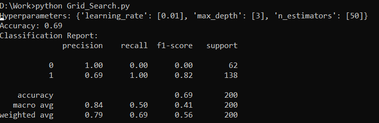
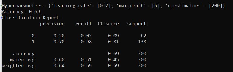
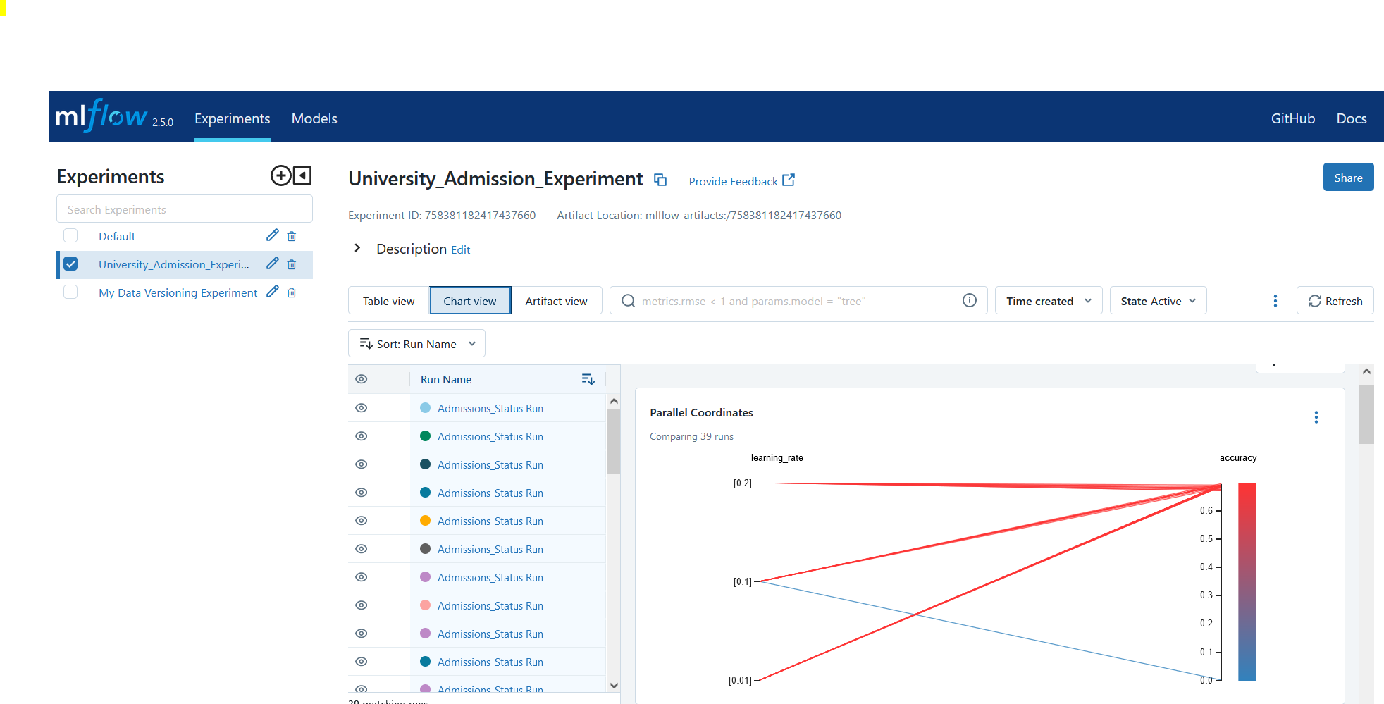
Here is the output on the MLflow server:

Conclusion
MLflow’s grid search tool automates tweaking, tracking the results, and modifying the hyperparameters in machine learning models. It helps to determine the ideal hyperparameters and ensures the reliable results but can be computationally expensive for extensive hyperparameter experiments.
Source: linuxhint.com