Google Sheets, a powerful spreadsheet tool, allows you to connect and utilize data from multiple sheets within the same document. This capability to reference data from one sheet to another streamlines data management, analysis, and presentation. By establishing links between sheets, you can effortlessly access and manipulate information across different sections of your spreadsheet, creating a more organized and effective data-handling process.

In this guide, we will discuss in detail two methods that can be utilized for creating references between different Sheets in Google spreadsheets: utilizing the IMPORTRANGE function and using Hyperlink.

Method 1: Utilizing the IMPORTRANGE Function

Data can be imported from one spreadsheet to another using the IMPORTRANGE function in Google Sheets, which is a strong tool. It is usually employed for importing data from other spreadsheets, but it can also be used to import data from one sheet to another inside the same spreadsheet.

Let’s go through the steps and details of using the IMPORTRANGE function to reference data from one sheet to another in Google Spreadsheets.

To begin with this method, we first have to make sure that both the source sheet and the destination sheet are open in the same document of Google Sheets document.

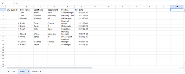
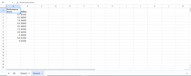
We currently have Sheet1 and Sheet2 open in the same Google spreadsheet. Sheet1 stores employees’ data, while Sheet2 contains additional details about employees.

Sheet1 looks like this:

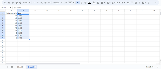
And Sheet2 has the following data stored in it:

Suppose we need to display column A, “Performance Score” of Sheet2 on Sheet1, so we can better analyze the data.

For this, we would reference the required column of Sheet2 to Sheet1.

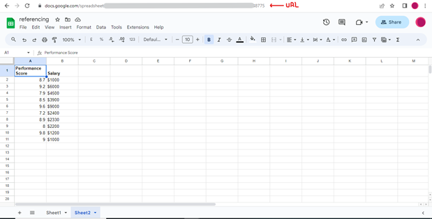
To utilize the IMPORTRANGE function, we need to have the URL of the Google Sheets document from which we want to reference a column. In your browser’s address bar, look for the URL for the Sheet when you’re viewing your spreadsheet and copy this URL.

Then go to the destination Sheet, which is Sheet1, and write the IMPORTRANGE function in the cell where you want to import the data from the source Sheet.

Here, we want to import a column from source Sheet Sheet2 into column G of the destination Sheet Sheet1. So, we clicked on cell G1 and wrote the IMPORTRANGE function.

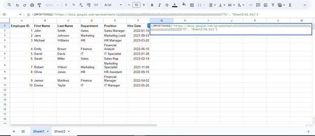
In this function, we first provided the source Sheet’s URL, which we copied earlier. Then specify the Sheet name, which in our case is Sheet2, and subsequently, provide the range of cells you want to import from the source. For instance, we want to import the data from cell A1 to A11 of Sheet2 to column G of the Sheet1.

When you enter the formula, Google Sheets will recognize that you’re trying to import data from another sheet. It will request permission to access the source spreadsheet, and you’ll need to grant permission for the import to work.

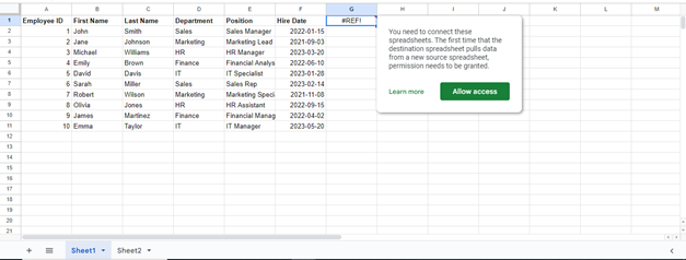
To grant the required authorizations, click the “Allow access” button. This authorization is necessary to protect the data’s privacy and security.

Once we’ve confirmed the import, the cell where we entered the IMPORTRANGE formula (i.e. G1) will now display the imported data (Performance score column) from the source sheet, which is Sheet2.

We need to remember that the imported data is dynamic; any changes you make to the source data in Sheet2 will be reflected in the destination sheet (Sheet1) after a short delay.

Method 2: Referencing with a Hyperlink

Referencing data from one sheet to another using a hyperlink in Google Sheets involves creating a hyperlink in a cell that, when clicked, takes you to a specific cell or range in another sheet.

Let’s create an example utilizing the above-generated data.

The first thing we must do here is select the cell where we need to create a hyperlink. Make sure you select the cell in the source sheet so you will be directed to the destination sheet when you click on it.

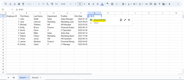
The source sheet, in our case, is Sheet1. We have selected cell G1, to create a destination link in it. Right-click on this cell, and a dropdown menu will appear.

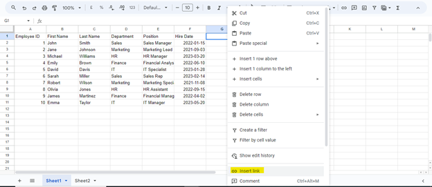
Choose “Insert link” from this menu. The dialogue pane that appears will have a “Sheets and named ranges” tab. This tab lets you link to a specific sheet and range within your spreadsheet.

Then select the target sheet you want to link to from the dropdown list. In our case, we have chosen Sheet2 as the target sheet. The target sheet is the sheet where the data we want to reference is located.

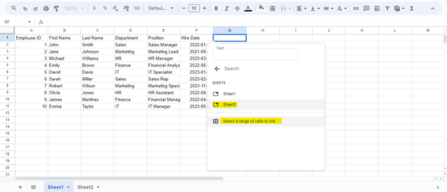
The target sheet’s specific cell or range can be set by hitting the “Select a range of cells to link” tap.

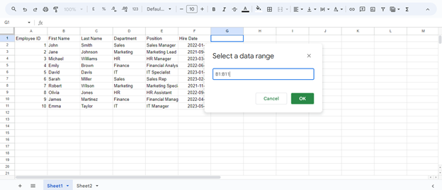
As we want to link the cell range B1:B11 from Sheet2, we have specified it in the “Select a data range” dialogue box.

After defining the target sheet and range, click the “OK” button. You will see the hyperlink text displayed in the selected cell.

As we click on the created hyperlink in the cell G1. This will take us to the specified cell or range in the target sheet, i.e., Sheet2!B1:B11, allowing us to view or work with the referenced data.

We have successfully referenced data from one sheet to another with a hyperlink. Using hyperlinks in this way provides an interactive and user-friendly method of referencing data between sheets in Google Sheets.

Conclusion

Referencing one sheet from another in Google Sheets is an essential technique. This article provided you with two methods that can be practiced to establish a connection between different sheets. The first method involves using the IMPORTRANGE method to provide seamless analysis of data by creating a reference between two sheets. The second method we discussed provides us with a hyperlink to establish a connection between the two specified sheets for sharing data. Both of these techniques are equally handy and implementable.