Google Sheets offers several helpful tools that can be used to organize and analyze data efficiently. One of these tools that is particularly useful for manipulating and extracting data is the FILTER function. Users can create customized representations of information without changing the original dataset by using the FILTER function to obtain data from a spreadsheet based on predefined criteria dynamically.

The Google Sheets FILTER tool allows users to isolate and work with subsets of data, making the process of analyzing and making decisions more efficient and instructive, whether you’re handling enormous datasets or simply want to display data more meaningfully.

Syntax
The following is syntax for using the FILTER function in Google Sheets:

Now let’s first understand this syntax.

The FILTER function typically has two parameters, which are range and conditions. The range indicates the cells we need to filter. A named range or a cell reference can be employed to specify it. At the same time, condition1 and condition2 are the requirements that the data in the provided range must meet for it to be included in the filtered result. Here, condition2 is an additional parameter.

This function can be applied to the provided dataset with either single or multiple conditions.

In this article, we will delve into both these methods to comprehend the utilization of the FILTER function in Google Sheets.

Table Creation

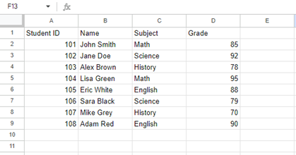
We will first create a sample table in a Google spreadsheet that we will use in the example throughout this article. So, we have constructed a table with four columns, where column A stores the Student ID, column B lists the students’ names, column C preserves the Subject, and column D holds the corresponding Grade.

Let’s start learning how to filter data from this table with single or multiple criteria.

Example 1: FILTER with Single Criteria in Google Sheets

The first illustration will work by utilizing the FILTER function with a single condition to retrieve some data from the above-generated table.

Let’s suppose we want to filter the record from the table where the student’s name is “Sarah Black”.

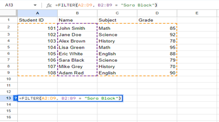
So, we clicked on the cell where we wanted to write the formula to filter out the specified record, which is cell A13 of the spreadsheet.

The formula we would write for this is as follows:

=FILTER(A2:D9, B2:B9 = “Sara Black”)

In this formula, A2:D9 is the range of cells from which the Google Sheets will search for the specified condition. This means that criteria will be looked for from cell A2 to the end of the table, which is cell D9. Then B2:B9 = “Sara Black” is the condition we have specified. The B2:B9 refers to the range of cells in column B, specifically from cell B2 to cell B9. Names are contained in these cells, as seen in the table. And “Sara Black” is a text value from which we want to retrieve the record.

So, B2:B9 = “Sara Black” will check each cell in the range B2:B9 to see if it equals “Sara Black“. If a cell in that range contains the text “Sara Black“, the result of this comparison will be displayed in that cell. If not, we will get an N/A, meaning no match is found.

So, to execute this formula, press the Enter key.

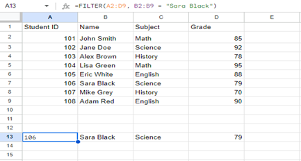
As shown in the above image, the condition has been met. The text “Sara Black” has been found, and the FILTER function returned the entire row of the data that meets the specified condition. We have the record for the name “Sara Black.”

Example 2: FILTER with Multiple Criteria in Google Sheets

Filtering with multiple criteria in Google Sheets involves utilizing logical operators like AND and OR to combine conditions.

Now we will create an instance where we will use both of these operators to filter multiple criteria in Google spreadsheets.

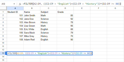
Suppose we want to filter the data based on two conditions: the Subject is either “English” or “History,” and the Grade is greater than or equal to 80. This is the formula we would use:

=FILTER(A2:D9, ((C2:C9 = “English”) + (C2:C9 = “History”)) * (D2:D9 >= 80))

Let’s comprehend this formula first.

In this formula, A2:D9 is the cell range. The (C2:9 = “English”) + (C2:C9 = “History”) check two conditions. The (C2:C10 = “English”) checks if the value in each cell of the “Subject” column (C2:C9) is equal to “English”. Whereas the part (C2:C10 = “History”) checks if the value in each cell of the “Subject” column (C2:C9) is equal to “History.” The (+) acts as a logical OR operator here. The (*) operator combines these two conditions using a logical AND. This indicates that a row cannot be contained in the filtered outcome unless both criteria are met. The (D2:D9 >= 80) checks if the grade listed in column D is 80 or above.

Simply put, the formula filters the data in the range A2:D9 based on the criteria that the subject must be “English” or “History”. Furthermore, the grade has to be greater or equal to 80.

When we hit Enter, rows that meet both of these conditions will be demonstrated in the filtered result.

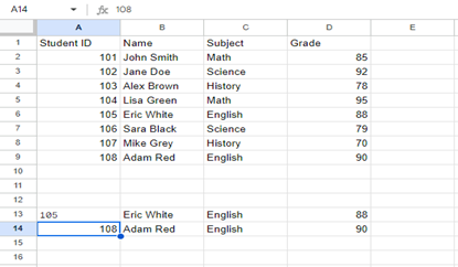
Here you can see that only two rows have met the specified conditions, which are for Student ID 105, and 108. The subject for both these records is “English,” with marks greater than 80.

This is a way to quickly find and display student records that match specific subjects and grade criteria from a larger dataset.

Conclusion

Using the FILTER function in Google Sheets is a very handy method for finding specified information from large amounts of data. You can use the FILTER function with a single criterion or with many conditions. We have performed the FILTER formula with single criteria in the first example, where we retrieved the record against a specified student name. At the same time, the multiple criteria procedure is elaborated in the second illustration, where we have filtered records based on two conditions.