The COUNTIF function within Google Sheets is a robust tool that enables you to tally the cells within a defined range that adheres to a given condition or criterion. This function proves especially valuable for filtering the data, conducting a fundamental data analysis, and acquiring insights from your spreadsheet.

This article explores on the instances where we can employ this formula to extract specific data records.

Syntax:

The syntax to use the COUNTIF function in Google Sheets is given as follows:

This function has two parameters: range and criteria. The range parameter refers to a set of cells that you want to count, and the criteria parameter signifies the condition that you’re applying to those cells.

To begin handily implementing this function, we first need to insert some data on which this function is applied to obtain the output.

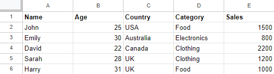
So, in our Google Sheets, we create a table and insert the data for five columns. Each column holds six entries.  Column A contains the names of people. Column B  shows their ages. Column C indicates their respective countries. Column D specifies the category that they belong to. And column E shows their sales in dollars.

In this table, we’ll provide some examples of using the COUNTIF function to count the data based on specific criteria.

Using COUNTIF for a Single Criterion

The COUNTIF function is particularly designed to count on a single criterion. Here, we will go through two examples to comprehend its usage in Google Sheets.

Example 1: Count the Occurrences of the USA Text in the Table

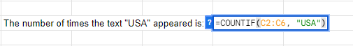
For the first illustration, we use the COUNTIF function to count the number of people that belong to USA or to count the appearance of the USA text in the table. The formula that we use for this is given as follows:

Now, let’s break it into the steps to understand it further.

The =COUNTIF is the keyword to use the COUNTIF formula. It indicates that we are using the COUNTIF formula to count the cells based on a particular provided criterion.

Within the function brackets, we specify the two parameters: range and criteria. In this case, the range that we specify is from cell C2 to C6 which corresponds to the Country column where you have different countries listed. The criteria (condition) that we aim to impose on the cells within the designated range is USA. So, here, we are looking for cells that contain the USA text.

When combined, the =COUNTIF(C2:C5, “USA”) formula directs the Google Sheets to tally the cells within the C2:C6 range that encompasses the USA text. Subsequently, it yields the tally of cells that fulfill this specific condition.

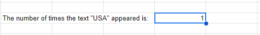
The COUNTIF function tallies and displays the output as we hit “Enter”. The following snapshot shows that the USA text appears only one time in the provided table:

Example 2: Count the Number of People Younger than Thirty

The next task that we perform using the COUNTIF function in Google Sheets is to count the number of people whose age is under 30.

The formula for this is:

Here, B2:B6 is the range, and the criteria is <30. Google Sheets scans the B2:B6 range and examines each cell’s numeric value (age). It counts the cells where the age is less than 30. And ultimately, the final count of cells that satisfy this condition is returned.

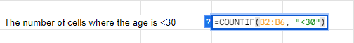
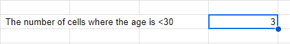
The =COUNTIF(B2:B6, “<30”) formula counts how many individuals have ages less than 30. Since there are three people (John, David, and Sarah) with ages less than 30 in the B2:B6 range, the formula yields a count of 3 which can be seen in the following image:

Using COUNTIFS for Multiple Criteria

We already mentioned that the COUNTIF formula is used for a single criterion only. But if we want to execute it to count the cells based on multiple criteria, we can utilize the COUNTIFS function. We simply it to continue adding the pairs of ranges and criteria as needed for the specific counting requirements.

Here, we provided you with two examples of utilizing the COUNTIFS formula in Google Sheets.

Example 3: Count the Number of Individuals Named “Harry” with Sales Below $1500

For this example, we have two criteria. The first one is to count the number of people with the name “Harry” and then a second criterion is to be applied which is to only count the number of those Harry whose sales is below $1500.

So, the formula that we have is:

In the A2:A5 range, i.e. the “Name” column, the name is Harry. Whereas, in the E2:E6 range, i.e. the Sales ($) column, the sales value is less than $1500.

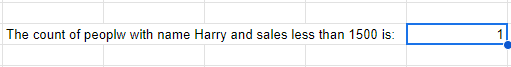
The formula counts the occurrences where both criteria are fulfilled simultaneously. In this case, only one occurrence meets both criteria: Harry’s entry with the sales of $1000.

So, the formula returns a count of 1 which can be seen in the following image:

Example 4: Count the Number of Individuals from the UK in the Food Category

This example also uses two criteria to count the specified condition from the provided cells.

The formula that we created with multiple criteria is:

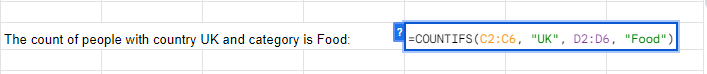
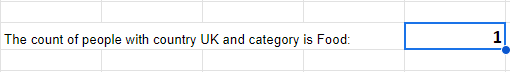
The formula calculates the instances where both conditions are met simultaneously: the country being the UK and the category being “Food”. In this particular scenario, only one occurrence aligns with both these criteria, i.e. Harry’s entry.

As a result, the formula yields a count of 1.

Conclusion

Using the COUNTIF function in Google Sheets is a beneficial technique. This article demonstrated some of the utilization of this function in a simple table to retrieve the number of records for the specified condition. Apart from using this formula for a single criterion, we have another form of this function: the COUNTIFS function which can be applied to retrieve the records that meet multiple criteria.  We provided you with four detailed examples in this guide to show these functions’ practical implementation and usage.