Conditional formatting is a functionality available in Google Sheets that allows altering cell appearance when specific criteria are fulfilled. This alteration can comprise various visual modifications such as highlighting, bold text, and italics. This capability extends beyond the current cell, enabling the application of conditional formatting based on conditions satisfied in different cells.

Table Creation

Making a table in Google Sheets is easy. Just follow these, steps for example:

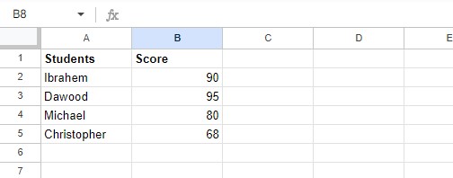
Start by forming a spreadsheet in Google Sheets with “four” rows and columns equal to “2”. This table will be used to show how conditional formatting can be done in Google Sheets. In the table, Column A is for students’ names, and Column B is for the grades or scores that record students’ performance in a specific subject. After entering the data in the columns, the spreadsheet will look the following way:

Now, we’ll work with this table that we have made to show conditional formatting in Google Sheets by implementing different easy-to-understand instances.

Example 1: Overview of Conditional Formatting on Google Sheets

Manual conditional formatting on Google spreadsheets requires the following basic steps:

Begin by selecting the group of cells we wish to apply the formatting rules to. Then, navigate to the “Format” option and choose “Conditional formatting.”

A window called “Conditional format rules” will pop up. Select the drop-down option or menu beneath “Format cells if…”

From here, pick the specific condition that will activate our rule. For the formatting style, decide on the visual changes we would prefer.

Conclude by clicking the “Done” button to implement the formatting.

Example 2: Conditional Formatting on Student’s Score Record

Now that we know how to apply conditional formatting in Google Sheets, let’s apply it to the real-world example for color coding grades.

We have a spreadsheet containing students’ names in column A and their corresponding test scores in column B. We want to visually highlight the students who scored above a certain threshold with a green color and those who scored below the threshold with a red color.

Here’s how we can achieve this using conditional formatting:

We have first selected the range, which means selecting the range of cells in column B that contain the test scores. Then to apply conditional formatting, go to the “Format” menu in the tool bar; from the format’s menu, choose “Conditional formatting.”

Once we have selected the conditional formatting option, a screen will appear to set the condition. From the panel of “Conditional Format Rules” which appears on the screen, select “Custom Formula is” Then we entered the formula:

=B2:B5 > 60

Here, we have assumed our threshold value to be 60. The formula will analyze whether cells B2 to B5 have a value greater or larger than 60.

After specifying the condition, we will choose the formatting style. Click on the “Formatting style” box and select the green color that we want to apply, which means if the condition met, i.e., B2:B5, is greater than 60, then the cell B2 will be highlighted with green color.

For an additional rule to handle scores below the threshold, click the “Add another rule” button in the “Conditional format rules” panel.

For setting the second condition, we would like to choose “Custom formula is” again and will enter a formula like “=B2:B5 <= 55”. The formula will inquire whether the cells B2:B5 hold a value less than or equal to 55.

We will again choose another formatting style for this second condition, and for this, we have selected the red color that we want to apply if the second condition meets.

To apply the rules after setting up both rules, click “Done.” The cells with scores above 60 will now be highlighted in green, while those below or equal to 55 will be highlighted in red.

Conditional formatting is a useful tool that changes how cells look based on certain rules. In this case, we made rules to see if a student’s score was high or low. The first rule highlighted scores above 60 in green, while the second highlighted scores below 60 in red. This helps us find the top and bottom scores without sorting or checking each one. It shows data in a way that helps us see patterns easily, which is great for big sets of data.

Example 3: Conditional Formatting for Budget Evaluation or Tracking

For this illustration, we will consider a scenario where Google Sheets monitors monthly expenditures.

The table will include three columns e.g., “Expense Category” in Column A, “Amount Spent”in Column B, and “Budget Limit” in Column C. The objective is to identify expenses exceeding the budget by highlighting them in red color using conditional formatting.

The first thing we need to do for applying conditional formatting is to select the range, so we will select the range of cells in Column B containing expense amounts.

To apply conditional formatting, access “Format” and opt for “Conditional formatting.”

We have specified the condition within “Conditional format rules,” choosing “Custom formula is.” And then insert the formula:
=B2:B4 > C2:C4

Where B2:B4 represents the spent amount and C2:C4 denotes the budget limit for the entire cells in the range.

Formatting Style will be selected, like a yellow background, to indicate expenses exceeding budget. Confirm the application of the rules by clicking “Done.”

If an expense in Column B exceeds its corresponding budget limit in Column C, the cell will change to yellow automatically, indicating overspending in that category. This method helps manage finances by promptly highlighting areas where budget limits are breached.
In this instance, conditional formatting facilitates precise financial management by promptly revealing instances of exceeding budgets within each category.

Conclusion

Throughout these examples, we’ve explored the practical application of conditional formatting in Google Sheets, from color-coding grades to managing expenses. This dynamic tool allows data to be visually represented in meaningful ways, assisting in identifying patterns quickly. By employing conditional formatting, we can enhance efficiency in decision-making and gain insights from our data effortlessly.